I don't ever blink, honestly. Ridley Scott

Massive artifacts like blinks and heart beats account for a large portion of variance in MEG data. They recur in the data and are usually stable in topography. ICA is a choice method to attempt removing these artifacts.

Prerequisite

MEG or EEG raw data has been acquired, along with EOG and/or EKG channels.

Major artifacts (large muscle contractions, subject moves, large electronic pop-off) have been marked in the data (see Detect and mark bad data segments).

Goal of this tutorial

Here we will compute an ICA of the data, and correlate the results with EOG and EKG channels. Components with correlation above a defined threshold will be selected. We inspect the results with and without these components and reject (or not!).

Step-by-step guide

If you are located within the CENIR, you can find scripts to perform these actions under /network/lustre/iss01/cenir/analyse/meeg/00_max/share/icapipe along with other useful tools. Elsewhere, you can download the scripts from https://gitlab.com/icm-institute/meg/icapipe.

In MATLAB, run the following code:

copyfile('/network/lustre/iss01/cenir/analyse/meeg/00_max/share/icapipe/pipe_icarej.m','/where/you/want/it/mypipe.m')

edit /where/you/want/it/mypipe.m
% don't forget to change /where/you/want/it/ above to the location where you want to store the pipeline (e.g. in your experiment's directory)

In the file you just copied, you will find the following code (after some initialization code, which you don't want to change):
```
file = '/network/lustre/iss01/cenir/analyse/meeg/00_max/share/example_data.fif'; % choose your MEG file

cfg  = [];
cfg.dataset = file;
cfg.channel = {'MEG' 'BIO*'}; % choose channels (include EOGs/ECGs...)
cfg.excludebad = 'yes';
[data, comp ] = do_ica(cfg);
```
exclude bad portions of signal

As mentioned earlier, you should remove (very) bad portions of signal before performing this step (with cfg.excludebad = 'yes'). To do this, follow instructions here.
The marker you use to mark bad segments of data has to be called "BAD".

Use SASICA to select components correlated with given channels

cfg  = [];
cfg.chancorr.enable = 1;    % enable the 'channel correlation' method of SASICA
cfg.chancorr.corthresh = .5;% correlation threshold is 0.5
cfg.chancorr.channames = {'BIO001','BIO002'};% the channels that should be used
%                       Any component that correlates with any of these
%                       channels above threshold will be returned in
%                       comps2del below.
% Other methods are available. Type doc eeg_SASICA in the command window for
% more information.

% SASICA opens a series of IC topographies. The selected ones have a red
% button below. Click on the button to see IC properties. Click "show
% subtraction" at the bottom of the window to show effect of subtraction on
% the time courses.
comps2del = ft_SASICA_neuromag(cfg,comp,data)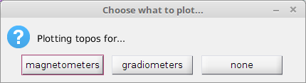

Select magnetometers or gradiometers (if you're not sure, just choose magnetometers)
These figures show up.
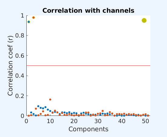
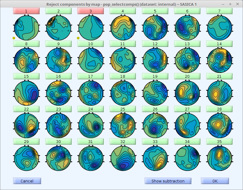
Any component that correlates with any of the channels entered in cfg.chancorr.channames above is highlighted in red. Click on the button of any component to examine the component's properties.
Component properties
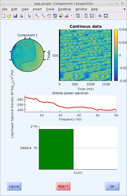
This figure shows the topography, time course, power spectrum and level of correlation (in number of times the specified threshold) for the selected component. Refer to the literature to decide which components to remove.
This paper can be helpful:
Other methods available

Other methods than correlation with selected channels are available, type doc eeg_SASICA in MATLAB to find out (more info in the paper).
Whether or not to reject a given component is left to you. Click the "Reject" button to toggle rejection status. Right click in the main figure to quickly toggle without looking at a component.

Subtract the components

cfg                           = [];
cfg.component                 = comps2del ;
data_corrected                = ft_rejectcomponent(cfg, comp, data );

Write the results to disk

In various formats as convenient to you...

[p,n,~] = fileparts(file) ;

component_filename = [p filesep n '_ica_comp.mat'];
save(component_filename,'comp');

output_filename = [ p filesep n '_ica_cor.fif' ];
fieldtrip2fiff( [ output_filename ], data_corrected );

Best is to work with the CENIR copy of this pipeline (see link above).

You can also download the repository, but you will need to also download https://github.com/fieldtrip/fieldtrip (or have a recent working copy of FieldTrip) and https://gitlab.com/icm-institute/meg/icapipe.git

Q&A

Including EOGs and ECGs in the ICA?

Yes, this improves separation. It "guides" the ICA and will push the components "up" in the plots (because they explain more variance).

Removing bad portions of signal?

This is always a good idea for non reproducible artifacts (movement, swallow...)

Downsample the data

Will improve speed. We have usually too much data. Resampling at 100 Hz should be ok.

How many components?

A bit of trial and error here. Asking for too many will prevent convergence (and is slow), too few will see a poor separation (but is quick). 2/3 of the rank of the data is in my experience a rough guide.

CENIR

Use ICA to subtract blink and cardiac activity