This is a collaborative space. In order to contribute, send an email to maximilien.chaumon@icm-institute.org
On any page, type the letter L on your keyboard to add a "Label" to the page, which will make search easier.
Single trials - Sources analysis
In this tutorial, you will find a description of all the steps necessary to obtain sources localisation of continuous (non averaged) data using a D.I.C.S beamformer approach in FieldTrip for one subject.
Prerequisites
- Read the previous tutorials (MEG EEG pre-processing, MEG sensors realignment, filter, baseline correction)
- Pre process the T1 MRI data or choose a template
- Download the latest version of FieldTrip - Install it in your software folder - Take a look at the FieldTrip tutorials!
Input data
MEG signals (MEG)
FieldTrip can import the fif files coming from our MEG system and those pre processed with our in-house tools. If you acquired simultaneous MEG+EEG data, FieldTrip will import both of them.
MRI
If you have the individual anatomy of each of your subjects (T1 MRI), you should process it with FieldTrip as described below.
If you don't have the individual anatomy, then you have to choose a template in FieldTrip.
Needed software
For MEG fif files pre processed outside FieldTrip: You will need two in-house scripts to read the marker files we add to the MEG fif files (put them in your matlab path):
A short script to pre process the MRI in FieldTrip: pre_process_mri_for_ft.m
A simple script to visualize beamformer results: visuBF.m
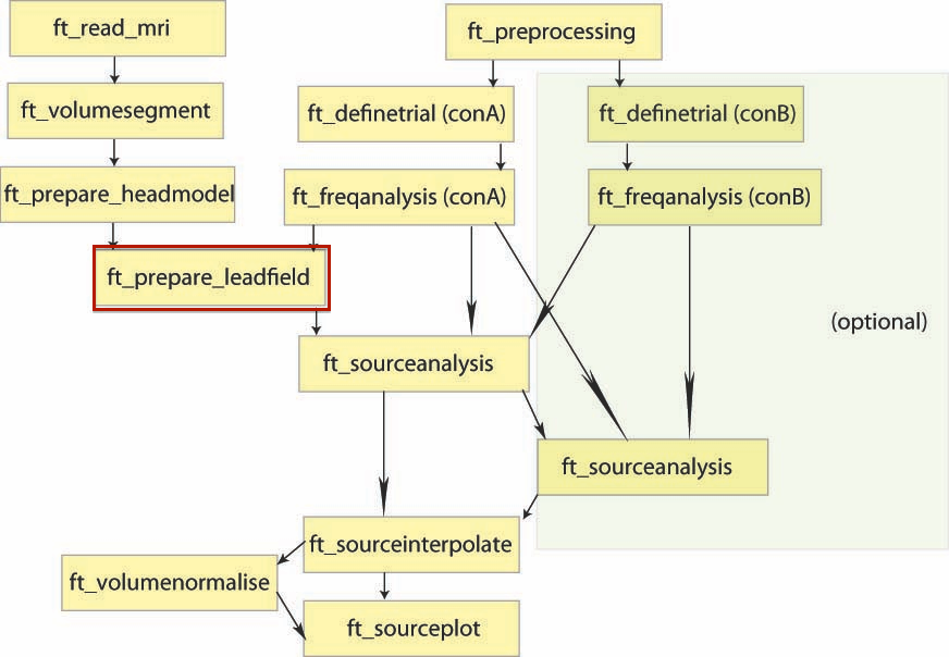
D.I.C.S. analysis with FieldTrip
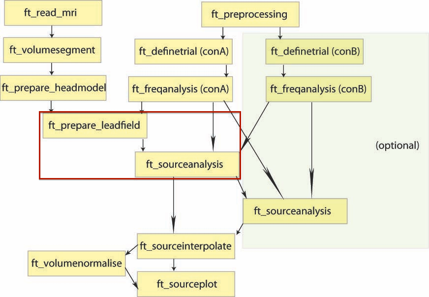
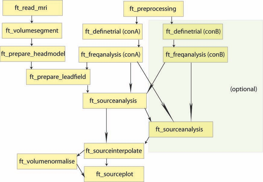
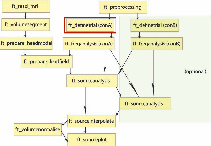
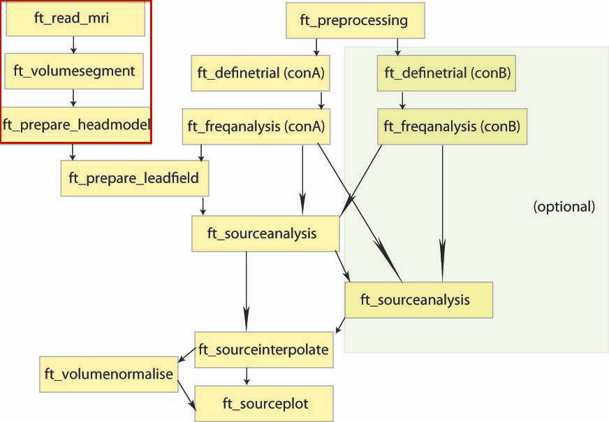
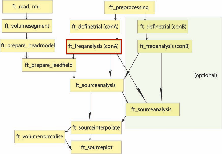
Overview of the process:
Suggested data organisation
The mat files generated by FieldTrip can be stored together with the pre-processed data. You may want to create a specific sub folder "FT" to store them in each subject.
Read data
The data should be pre processed (i.e. artefact free) at this point and the FieldTrip folder in your matlab path.
MEG data
ft_defaults ; %% Load fieldtrip configuration

%% Read two runs, define trials around LEFT_MVT_CLEAN marker (-2s to 2s around the marker), read also BIO005 which is an EMG.
[ trials ] = trial_definition_ft( {'cardiocor_blinkcor_run03_tsss.fif' 'cardiocor_blinkcor_run04_tsss.fif'}, 'LEFT_MVT_CLEAN', 2.0, 2.0, 'BIO005' ) ;
MRI processing
This step has to be done only one time. Provide the file name of you T1 MRI exam (can be nifty format for instance). The results will loaded as needed in the coming analysis.
mri=ft_read_mri(file_name);
%% Realign the MRI to the MEG coordinate
cfg=[];
cfg.method = 'interactive' ;
cfg.coordsys = 'neuromag' ;
mri_aligned = ft_volumerealign(cfg,mri) ;

save('mri_aligned.mat', 'mri_aligned');

%% Segmentation
cfg           = [];
cfg.output    = 'brain';
segmentedmri  = ft_volumesegment(cfg, mri_aligned);

save('segmentedmri.mat', 'segmentedmri') ;


% construct volume conductor model (i.e. head model) for each subject
cfg = [];
cfg.method = 'singleshell';
vol = ft_prepare_headmodel(cfg, seg);
vol = ft_convert_units(vol, 'cm');
save('vol.mat', 'vol') ;
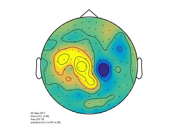
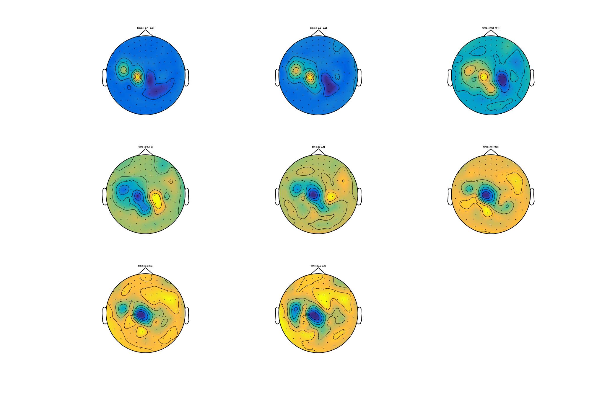
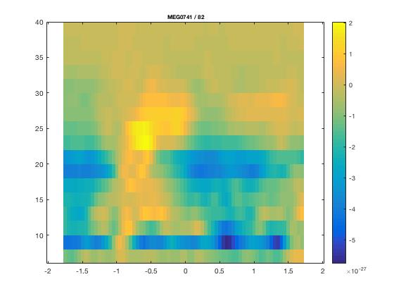
Time-Frequency analysis
cfg              = [];
cfg.output       = 'pow';
cfg.channel      = 'MEG';
cfg.method       = 'mtmconvol';
cfg.taper        = 'hanning';
cfg.foi          = 7:2:40;                         % analysis 2 to 30 Hz in steps of 2 Hz
cfg.t_ftimwin    = ones(length(cfg.foi),1).*0.5;   % length of time window = 0.5 sec
cfg.toi          = -2.0:0.05:2.0;                  % time window "slides" from -2.0 to 2.0 sec in steps of 0.05 sec (50 ms)
cfg.trials       = 'all';

TFRhann = ft_freqanalysis(cfg, full_data_all);

%% Visualization
cfg = [];
cfg.xlim = [0.1 0.2];
cfg.ylim = [20 20];
cfg.zlim = [-1e-28 1e-28];
cfg.baseline     = [-0.2 -0.0];
cfg.baselinetype = 'absolute';
cfg.layout       = 'neuromag306mag.lay';

figure; ft_topoplotTFR(cfg,TFRhann);

% for the multiple plots also:
cfg = [];
cfg.ylim = [20 20];
cfg.baseline     = [-0.2 -0.0];
cfg.baselinetype = 'absolute';
cfg.layout       = 'neuromag306mag.lay';
cfg.xlim = [-0.4:0.1:0.4];
cfg.comment = 'xlim';
cfg.commentpos = 'title';
figure; ft_topoplotTFR(cfg,TFRhann);

cfg = [];
cfg.baseline     = [-1.0 -0.8];
cfg.baselinetype = 'absolute';
%% cfg.zlim         = [-1e-27 1e-27];
cfg.showlabels   = 'yes';
cfg.layout       = 'neuromag306mag.lay';
figure; ft_multiplotTFR(cfg, TFRhann);
CSD Computation
cfg = [];
cfg.channel      = 'meg' ;
cfg.pad          = 'nextpow2';
cfg.method       = 'mtmfft';
cfg.output       = 'powandcsd';
cfg.keeptrials   = 'no';
cfg.foi          = freqofinterest ;
cfg.tapsmofrq    = freqhalfwin ;

%% Compute cross-sepctral density matrices
powcsd_all = ft_freqanalysis(cfg, data_all) ;
powcsd_active = ft_freqanalysis(cfg, data_timewindow_active) ;
powcsd_ref = ft_freqanalysis(cfg, data_timewindow_ref) ;
Forward operator
We compute the lead field based on the warped MNI grid.
% Create leadfield grid
cfg                 = [];
cfg.channel         = channelsofinterest ;
cfg.grad            = powcsd_active.grad;
cfg.vol             = vol ;
cfg.dics.reducerank = 2; % default for MEG is 2, for EEG is 3
cfg.grid.resolution = 1.0;   % use a 3-D grid with a 0.5 cm resolution
cfg.grid.unit       = 'cm';
cfg.grid.tight      = 'yes';
cfg.normalize       =  lead_field_depth_normalization ; %% Depth normalization
[grid] = ft_prepare_leadfield(cfg);
D.I.C.S. Analysis
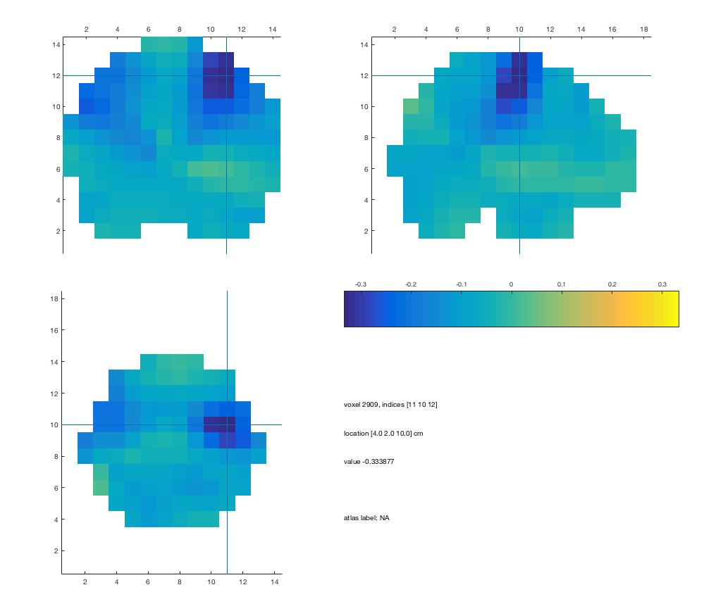
The spatial filters are computed here. We then contrast the two conditions before saving the results.
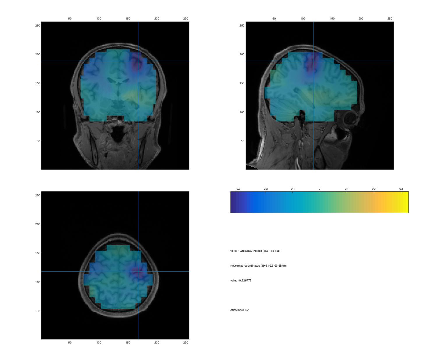
%% Compute DICS filters for the concatenated data
cfg              = [];
cfg.channel      = channelsofinterest ;
cfg.method       = 'dics';
cfg.frequency    = freqofinterest ;
cfg.grid         = grid;
cfg.headmodel    = vol;
cfg.senstype     = 'MEG';
cfg.dics.keepfilter   = 'yes'; % We wish to use the calculated filter later on
cfg.dics.projectnoise = 'yes';
cfg.dics.lambda  = beamformer_lambda_normalization;
source_all = ft_sourceanalysis(cfg, powcsd_all);

%% Apply computed filters to each active and reference windows
cfg              = [];
cfg.channel      = channelsofinterest ;
cfg.method       = 'dics';
cfg.frequency    = freqofinterest ;
cfg.grid         = grid;
cfg.grid.filter  = source_all.avg.filter;
cfg.dics.projectnoise = 'yes';
cfg.headmodel          = vol;
cfg.dics.lambda  = beamformer_lambda_normalization ;
cfg.senstype     ='MEG' ;

%% Source analysis active
source_active = ft_sourceanalysis(cfg, powcsd_active);

%% Source analysis reference
source_reference = ft_sourceanalysis(cfg, powcsd_ref);

%% Compute differences (power) between active and reference
source_diff = source_active ;
source_diff.avg.pow  = (source_active.avg.pow - source_reference.avg.pow) ./ (source_active.avg.pow + source_reference.avg.pow);

%% Display the results
visuBF( source_diff, 'title' )
%% MRI reslicing

mri_resliced = ft_volumereslice([], mri_aligned);

%% Display results superimposed on MRI

cfg            = [];
cfg.parameter = 'avg.pow';
source_active_int  = ft_sourceinterpolate(cfg, source_active, mri_resliced);
source_reference_int  = ft_sourceinterpolate(cfg, source_reference, mri_resliced);
source_diff_int  = source_active_int;
source_diff_int.pow  = (source_active_int.pow - source_reference_int.pow) ./ (source_active_int.pow + source_reference_int.pow);

%% Display the results
visuBF( source_diff_int, 'title' )