This is a collaborative space. In order to contribute, send an email to maximilien.chaumon@icm-institute.org
On any page, type the letter L on your keyboard to add a "Label" to the page, which will make search easier.
Combining MAG and GRAD with D.I.C.S
- Former user (Deleted)
- Maximilien CHAUMON
WARNING
This is not a tutorial - We are evaluating several ways to combine MAG and GRAD in the localisation process. You will find here the results we got with a D.I.C.S approach in FieldTrip
Prerequisites
- Read the previous tutorials (MEG EEG pre-processing, MEG sensors realignment, filter, baseline correction)
- Pre process the T1 MRI data or choose a template
- Download the latest version of FieldTrip - Install it in your software folder - Take a look at the FieldTrip tutorials!
Input data
MEG signals (MEG)
Here we will use simple MEG signals involving a grasping of the left hand (100 times).
MRI
We will use the MRI of the subject
Needed software
For MEG fif files pre processed outside FieldTrip: You will need two in-house scripts to read the marker files we add to the MEG fif files (put them in your matlab path):
A short script to pre process the MRI in FieldTrip: pre_process_mri_for_ft.m
A simple script to visualize beamformer results: visuBF.m
D.I.C.S. analysis with FieldTrip
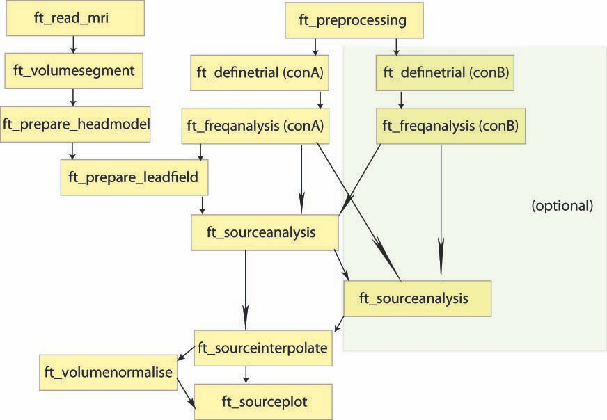
Overview of the process:
Goal of the tests
Evaluate the effects of mixing information from different kinds of sensors during the localisation process.
We will first show the simplest way to achieve that by insuring that every measurement is expressed in standard SI unit (i.e. meter) based on this discussion in the Fieldtrip mailing list:
i would suggest updating to a recent fieldtrip version. combining mags
and grads has been implemented there and you basically do not need to do
any extra steps. there are just these three pitfalls that you need to
pay attention to because it might lead to wrong results:

 1. make sure that you put in the original data. i.e. no prescaling etc.
    also make sure that you have not modified the .tra matrix of your
    grad structure.
 2. always compute your own leadfield. i.e. always use
    ft_prepare_leadfield to compute the forward model and don't have it
    done by ft_sourceanalysis. i don't know if this is absolutely
    necessary but as the ft_prepare_leadfield step is the one in which
    the actual pitfalls are, i would strongly suggest you do it
    separately to have maximum control!
 3. all the data going into ft_prepare_leadfield MUST BE in meters! i.e.:
     1. the grid mus be either created directly in meters of converted
        to meters by using ft_convert_unit
     2. the grad structure of your data must have been converted to
        meters. this is something you must do manually as according to
        my experience, fieldtrip does not take care of it. additionally,
        the default grad returned by ft_read_sens (and thus the one
        placed in your data structure) is in centimeters! so, it is a
        good idea to do something like this: data.grad =
        ft_convert_data(data.grad, 'm'); right after getting your data
        via ft_preprocessing!
     3. if you provide your grad structure in the cfg structure, also
        make sure that it is in meters.

the meters stuff is really extremely important!!! if your units are
wrong, you are going to end up with wrong source projections and will
not get an error message!!!

if you see some fieldtrip output like: "converting XXX to cm", your
results will be wrong!

if you take care of all that, fieldtrip does the scaling automatically
based on the distance between the two parts of each gradiometer.
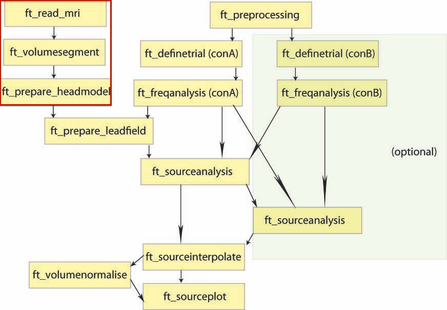
MRI processing
This step was done before (see previous tutorials). The results (aligned and segmented MRI, head model) will be loaded when needed.
D.I.C.S. Analysis
The spatial filters are computed here. We then contrast the two conditions before saving the results. We will do the localisation with both MAG & GRAD then MAG alone and to finish GRAD alone
Specific steps
We will convert sensors coordinates to meters and generate a grid in meters
channelsofinterest_meters = {'MEG'} ; %% MAG + GRAD are selected
powcsd_all = compute_crosprect(channelsofinterest_meters, freqofinterest, freqhalfwin, data_all) ;
powcsd_active = compute_crosprect(channelsofinterest_meters, freqofinterest, freqhalfwin, data_timewindow_active) ;
powcsd_ref = compute_crosprect(channelsofinterest_meters, freqofinterest, freqhalfwin, data_timewindow_ref) ;
%% Convert the grad structure to meters (I do that in the cross spectrum matrix to speed the test, should be done at the very beginning on the data itself
powcsd_all_meters = powcsd_all ;
powcsd_active_meters = powcsd_active ;
powcsd_ref_meters = powcsd_ref ;
powcsd_all_meters.grad = ft_convert_units(powcsd_all.grad, 'm') ;
powcsd_active_meters.grad = powcsd_all_meters.grad ;
powcsd_ref_meters.grad = powcsd_all_meters.grad ;
% Create leadfield grid
cfg = [];
cfg.channel = channelsofinterest_meters ;
cfg.grad = powcsd_active_meters.grad;
cfg.vol = vol ;
cfg.dics.reducerank = 2; % default for MEG is 2, for EEG is 3
cfg.grid.resolution = 0.01; %% should be in meter now ...
cfg.grid.unit = 'm';
cfg.grid.tight = 'yes';
cfg.normalize = lead_field_depth_normalization ; %% Depth normalization
[grid_meters] = ft_prepare_leadfield(cfg);
%% %%%%%%%%%% DICS %%%%%%%%%%
%% Compute DICS filters for the concatenated data
cfg = [];
cfg.channel = channelsofinterest_meters ;
cfg.method = 'dics';
cfg.frequency = freqofinterest ;
cfg.grid = grid_meters;
cfg.headmodel = vol;
cfg.senstype = 'MEG'; %
cfg.dics.keepfilter = 'yes'; % We wish to use the calculated filter later on
cfg.dics.projectnoise = 'yes';
cfg.dics.lambda = beamformer_lambda_normalization;
source_all_meters = ft_sourceanalysis(cfg, powcsd_all_meters);
%% Apply computed filters to each active and reference windows
cfg = [];
cfg.channel = channelsofinterest_meters ;
cfg.method = 'dics';
cfg.frequency = freqofinterest ;
cfg.grid = grid_meters;
cfg.grid.filter = source_all_meters.avg.filter;
cfg.dics.projectnoise = 'yes';
cfg.headmodel = vol;
cfg.dics.lambda = beamformer_lambda_normalization ;
cfg.senstype ='MEG' ;
%% Source analysis active
source_active_meters = ft_sourceanalysis(cfg, powcsd_active_meters);
%% Source analysis reference
source_reference_meters = ft_sourceanalysis(cfg, powcsd_ref_meters);
%% Compute differences (power) between active and reference
source_diff_meters = source_active_meters ;
source_diff_meters.avg.pow = (source_active_meters.avg.pow - source_reference_meters.avg.pow) ./ (source_active_meters.avg.pow + source_reference_meters.avg.pow);
%% Display the results
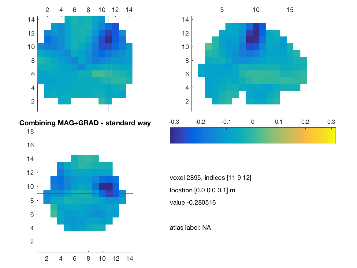
visuBF( source_diff_meters, 'title' )
title(['Combining MAG+GRAD - standard way']) ;
print(['comb_mag_grad_standard'],'-dpng')
channelsofinterest_meters = {'MEG*1'} ; %% Magnetometer on an Elekta system
powcsd_all = compute_crosprect(channelsofinterest_meters, freqofinterest, freqhalfwin, data_all) ;
powcsd_active = compute_crosprect(channelsofinterest_meters, freqofinterest, freqhalfwin, data_timewindow_active) ;
powcsd_ref = compute_crosprect(channelsofinterest_meters, freqofinterest, freqhalfwin, data_timewindow_ref) ;
%% Convert the grad structure to meters
powcsd_all_meters = powcsd_all ;
powcsd_active_meters = powcsd_active ;
powcsd_ref_meters = powcsd_ref ;
powcsd_all_meters.grad = ft_convert_units(powcsd_all.grad, 'm') ;
powcsd_active_meters.grad = powcsd_all_meters.grad ;
powcsd_ref_meters.grad = powcsd_all_meters.grad ;
% Create leadfield grid
cfg = [];
cfg.channel = channelsofinterest_meters ;
cfg.grad = powcsd_active_meters.grad;
cfg.vol = vol ;
cfg.dics.reducerank = 2; % default for MEG is 2, for EEG is 3
cfg.grid.resolution = 0.01; % use a 3-D grid with a 0.5 cm resolution %% I sippose this should be in meter now ...
cfg.grid.unit = 'm';
cfg.grid.tight = 'yes';
cfg.normalize = lead_field_depth_normalization ; %% Depth normalization
[grid_meters] = ft_prepare_leadfield(cfg);
%% %%%%%%%%%% DICS %%%%%%%%%%
%% Compute DICS filters for the concatenated data
cfg = [];
cfg.channel = channelsofinterest_meters ;
cfg.method = 'dics';
cfg.frequency = freqofinterest ;
cfg.grid = grid_meters;
cfg.headmodel = vol;
cfg.senstype = 'MEG'; % Must me 'MEG'
cfg.dics.keepfilter = 'yes'; % We wish to use the calculated filter later on
cfg.dics.projectnoise = 'yes';
cfg.dics.lambda = beamformer_lambda_normalization;
source_all_meters = ft_sourceanalysis(cfg, powcsd_all_meters);
%% Apply computed filters to each active and reference windows
cfg = [];
cfg.channel = channelsofinterest_meters ;
cfg.method = 'dics';
cfg.frequency = freqofinterest ;
cfg.grid = grid_meters;
cfg.grid.filter = source_all_meters.avg.filter;
cfg.dics.projectnoise = 'yes';
cfg.headmodel = vol;
cfg.dics.lambda = beamformer_lambda_normalization ;
cfg.senstype ='MEG' ;
%% Source analysis active
source_active_meters = ft_sourceanalysis(cfg, powcsd_active_meters);
%% Source analysis reference
source_reference_meters = ft_sourceanalysis(cfg, powcsd_ref_meters);
%% Compute differences (power) between active and reference
source_diff_meters = source_active_meters ;
source_diff_meters.avg.pow = (source_active_meters.avg.pow - source_reference_meters.avg.pow) ./ (source_active_meters.avg.pow + source_reference_meters.avg.pow);
%% Display the results
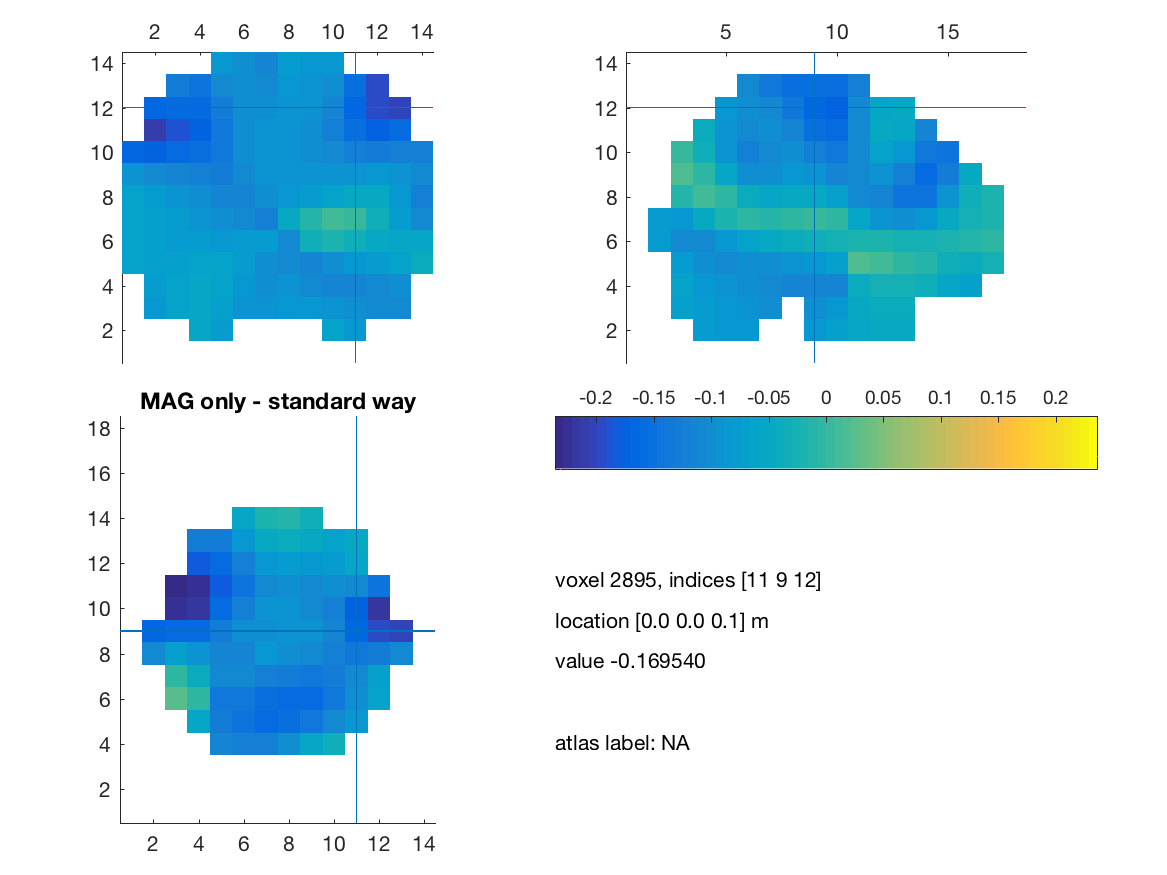
visuBF( source_diff_meters, 'title' )
title(['MAG only - standard way']) ;
print(['comb_mag_only_standard'],'-dpng')
channelsofinterest_meters = {'MEG*2', 'MEG*3'}; %% Gradiometers on an Elekta system

powcsd_all = compute_crosprect(channelsofinterest_meters, freqofinterest, freqhalfwin, data_all) ;
powcsd_active = compute_crosprect(channelsofinterest_meters, freqofinterest, freqhalfwin, data_timewindow_active) ;
powcsd_ref = compute_crosprect(channelsofinterest_meters, freqofinterest, freqhalfwin, data_timewindow_ref) ;

%% Convert the grad structure to meters
powcsd_all_meters = powcsd_all ;
powcsd_active_meters = powcsd_active ;
powcsd_ref_meters = powcsd_ref ;

powcsd_all_meters.grad = ft_convert_units(powcsd_all.grad, 'm') ;
powcsd_active_meters.grad = powcsd_all_meters.grad ;
powcsd_ref_meters.grad = powcsd_all_meters.grad ;

% Create leadfield grid
cfg                 = [];
cfg.channel         = channelsofinterest_meters ;
cfg.grad            = powcsd_active_meters.grad;
cfg.vol             = vol ;
cfg.dics.reducerank = 2; % default for MEG is 2, for EEG is 3
cfg.grid.resolution = 0.01;   % use a 3-D grid with a 0.5 cm resolution %% I sippose this should be in meter now ...
cfg.grid.unit       = 'm';
cfg.grid.tight      = 'yes';
cfg.normalize       =  lead_field_depth_normalization ; %% Depth normalization
[grid_meters] = ft_prepare_leadfield(cfg);

%% %%%%%%%%%% DICS %%%%%%%%%%
%% Compute DICS filters for the concatenated data

cfg              = [];
cfg.channel      = channelsofinterest_meters ;
cfg.method       = 'dics';
cfg.frequency    = freqofinterest ;
cfg.grid         = grid_meters;
cfg.headmodel    = vol;
cfg.senstype     = 'MEG';
cfg.dics.keepfilter   = 'yes'; % We wish to use the calculated filter later on
cfg.dics.projectnoise = 'yes';
cfg.dics.lambda  = beamformer_lambda_normalization;
source_all_meters = ft_sourceanalysis(cfg, powcsd_all_meters);

%% Apply computed filters to each active and reference windows
cfg              = [];
cfg.channel      = channelsofinterest_meters ;
cfg.method       = 'dics';
cfg.frequency    = freqofinterest ;
cfg.grid         = grid_meters;
cfg.grid.filter  = source_all_meters.avg.filter;
cfg.dics.projectnoise = 'yes';
cfg.headmodel          = vol;
cfg.dics.lambda  = beamformer_lambda_normalization ;
cfg.senstype     ='MEG' ;

%% Source analysis active
source_active_meters = ft_sourceanalysis(cfg, powcsd_active_meters);

%% Source analysis reference
source_reference_meters = ft_sourceanalysis(cfg, powcsd_ref_meters);

%% Compute differences (power) between active and reference
source_diff_meters = source_active_meters ;
source_diff_meters.avg.pow  = (source_active_meters.avg.pow - source_reference_meters.avg.pow) ./ (source_active_meters.avg.pow + source_reference_meters.avg.pow);

%% Display the results
visuBF( source_diff_meters, 'title' )
title(['GRAD only - standard way']) ;
print(['comb_grad_only_standard'],'-dpng')

ft_defaults
[ trials ] = trial_definition_ft( {'cardiocor_blinkcor_run03_tsss.fif' 'cardiocor_blinkcor_run04_tsss.fif'}, 'LEFT_MVT_CLEAN', 2.0, 2.0, 'BIO005' ) ;
%% %% Basic configuration
overall_time_window = [-2 2] ; %% if you modify this modify the trials def above !
active_time_window = [0.2 0.6] ;
reference_time_window = [-1.4 -1.0] ;
beamformer_lambda_normalization = '10%' ;
lead_field_depth_normalization = 'column' ;
freqofinterest = 22 ;
freqhalfwin = 6 ;
load vol ; %% load head model
load('mri_aligned.mat') ; %% MRI data needed for vizualisation
load('segmentedmri.mat') ;
% Select time window of interest
cfg = [];
cfg.toilim = active_time_window ;
data_timewindow_active = ft_redefinetrial(cfg,trials);
% Select time window of control
cfg = [];
cfg.toilim = reference_time_window ;
data_timewindow_ref = ft_redefinetrial(cfg,trials);
% Concatenate for common spatial filter
data_all = ft_appenddata([], data_timewindow_active, data_timewindow_ref);
channelsofinterest_meters = {'MEG'} ; %% Magnetometer on an Elekta system
%%%%%%%%%%%%%%%%%%%%%%%%%%%%%%%%%%%%%%%%%%%%%%%%%%%%%%%%%%%%%%%%%%%%%%%%%%
%% DICS Analysis combining both gradiometers and magnetometers in meter %%
%%%%%%%%%%%%%%%%%%%%%%%%%%%%%%%%%%%%%%%%%%%%%%%%%%%%%%%%%%%%%%%%%%%%%%%%%%
%% Select MAG + GRAD sensors
channelsofinterest_meters = {'MEG'} ; %% Magnetometer on an Elekta system
powcsd_all = compute_crosprect(channelsofinterest_meters, freqofinterest, freqhalfwin, data_all) ;
powcsd_active = compute_crosprect(channelsofinterest_meters, freqofinterest, freqhalfwin, data_timewindow_active) ;
powcsd_ref = compute_crosprect(channelsofinterest_meters, freqofinterest, freqhalfwin, data_timewindow_ref) ;
%% Convert the grad structure to meters (I do that in the cross spectrum matrix to speed the test, should be done at the very beginning on the data itself
powcsd_all_meters = powcsd_all ;
powcsd_active_meters = powcsd_active ;
powcsd_ref_meters = powcsd_ref ;
powcsd_all_meters.grad = ft_convert_units(powcsd_all.grad, 'm') ;
powcsd_active_meters.grad = powcsd_all_meters.grad ;
powcsd_ref_meters.grad = powcsd_all_meters.grad ;
%% NO peculiar weighting for the MAG (Sarang way)
wheigthing_coefficient = 1.0 ;
%% Convert the grad structure to meters
powcsd_all_meters = powcsd_all ;
powcsd_active_meters = powcsd_active ;
powcsd_ref_meters = powcsd_ref ;
powcsd_all_meters.grad = ft_convert_units(powcsd_all.grad, 'm') ;
powcsd_active_meters.grad = powcsd_all_meters.grad ;
powcsd_ref_meters.grad = powcsd_all_meters.grad ;
%% Lets tripote the covariance matrix (with the help of Sarang) - I put to zeros all the crossterms between mag and grad
for (i_dipole=1:length(powcsd_active_meters.labelcmb))
if powcsd_active.labelcmb{i_dipole,1}(end) == '1' %% its a mag
if powcsd_active.labelcmb{i_dipole,2}(end) == '2' | powcsd_active.labelcmb{i_dipole,2}(end) == '3' %% its a grad
powcsd_all_meters.crsspctrm(i_dipole) = 0.0 ;
powcsd_active_meters.crsspctrm(i_dipole) = 0.0 ;
powcsd_ref_meters.crsspctrm(i_dipole) = 0.0 ;
else
powcsd_all_meters.crsspctrm(i_dipole) = powcsd_all_meters.crsspctrm(i_dipole) * wheigthing_coefficient ;
powcsd_active_meters.crsspctrm(i_dipole) = powcsd_active_meters.crsspctrm(i_dipole) * wheigthing_coefficient ;
powcsd_ref_meters.crsspctrm(i_dipole) = powcsd_ref_meters.crsspctrm(i_dipole) * wheigthing_coefficient ;
end
else %% its a grad
if powcsd_active.labelcmb{i_dipole,2}(end) == '1' %% its a mag
powcsd_all_meters.crsspctrm(i_dipole) = 0.0 ;
powcsd_active_meters.crsspctrm(i_dipole) = 0.0 ;
powcsd_ref_meters.crsspctrm(i_dipole) = 0.0 ;
end
end
end
% Create leadfield grid
cfg = [];
cfg.channel = channelsofinterest_meters ;
cfg.grad = powcsd_active_meters.grad;
cfg.vol = vol ;
cfg.dics.reducerank = 2; % default for MEG is 2, for EEG is 3
cfg.grid.resolution = 0.01;
cfg.grid.unit = 'm';
cfg.grid.tight = 'yes';
cfg.normalize = lead_field_depth_normalization ; %% Depth normalization
[grid_meters] = ft_prepare_leadfield(cfg);
%% %%%%%%%%%% DICS %%%%%%%%%%
%% Compute DICS filters for the concatenated data
cfg = [];
cfg.channel = channelsofinterest_meters ;
cfg.method = 'dics';
cfg.frequency = freqofinterest ;
cfg.grid = grid_meters;
cfg.headmodel = vol;
cfg.senstype = 'MEG'; % Must me 'MEG', although we only kept MEG channels, information on EEG channels is still present in data
cfg.dics.keepfilter = 'yes'; % We wish to use the calculated filter later on
cfg.dics.projectnoise = 'yes';
cfg.dics.lambda = beamformer_lambda_normalization;
source_all_meters = ft_sourceanalysis(cfg, powcsd_all_meters);
%% Apply computed filters to each active and reference windows
cfg = [];
cfg.channel = channelsofinterest_meters ;
cfg.method = 'dics';
cfg.frequency = freqofinterest ;
cfg.grid = grid_meters;
cfg.grid.filter = source_all_meters.avg.filter;
cfg.dics.projectnoise = 'yes';
cfg.headmodel = vol;
cfg.dics.lambda = beamformer_lambda_normalization ;
cfg.senstype ='MEG' ;
%% Source analysis active
source_active_meters = ft_sourceanalysis(cfg, powcsd_active_meters);
%% Source analysis reference
source_reference_meters = ft_sourceanalysis(cfg, powcsd_ref_meters);
%% Compute differences (power) between active and reference
source_diff_meters = source_active_meters ;
source_diff_meters.avg.pow = (source_active_meters.avg.pow - source_reference_meters.avg.pow) ./ (source_active_meters.avg.pow + source_reference_meters.avg.pow);
%% Display the results
visuBF( source_diff_meters, 'title' )
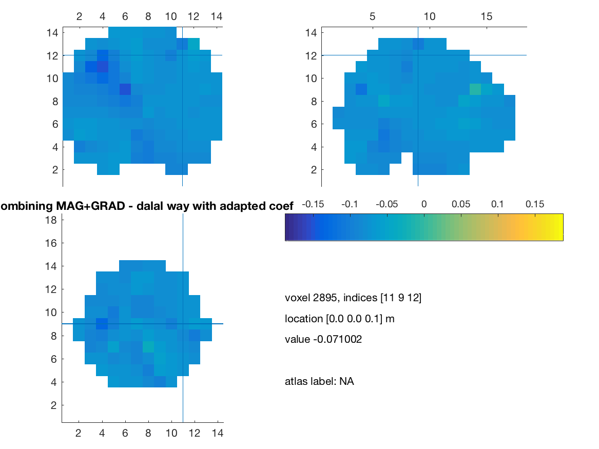
title(['Combining MAG+GRAD - dalal way']) ;
print(['comb_mag_grad_dalal'],'-dpng')

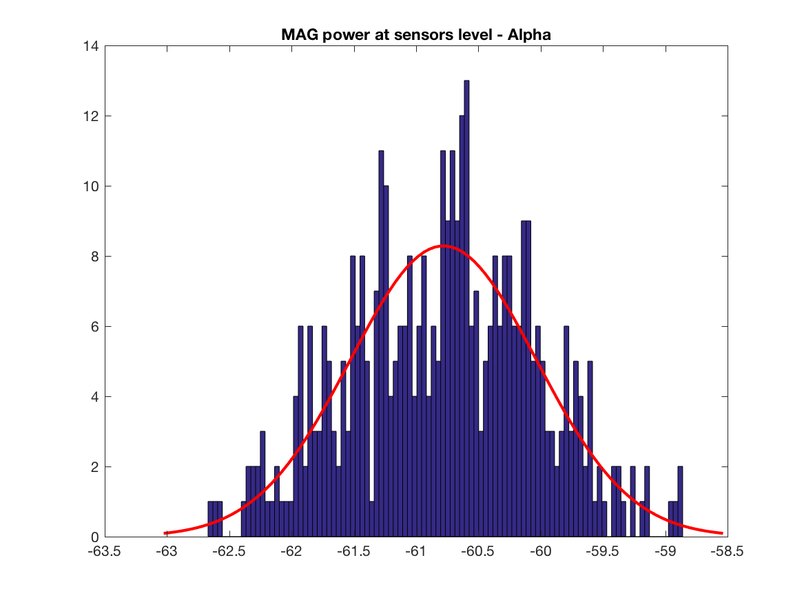
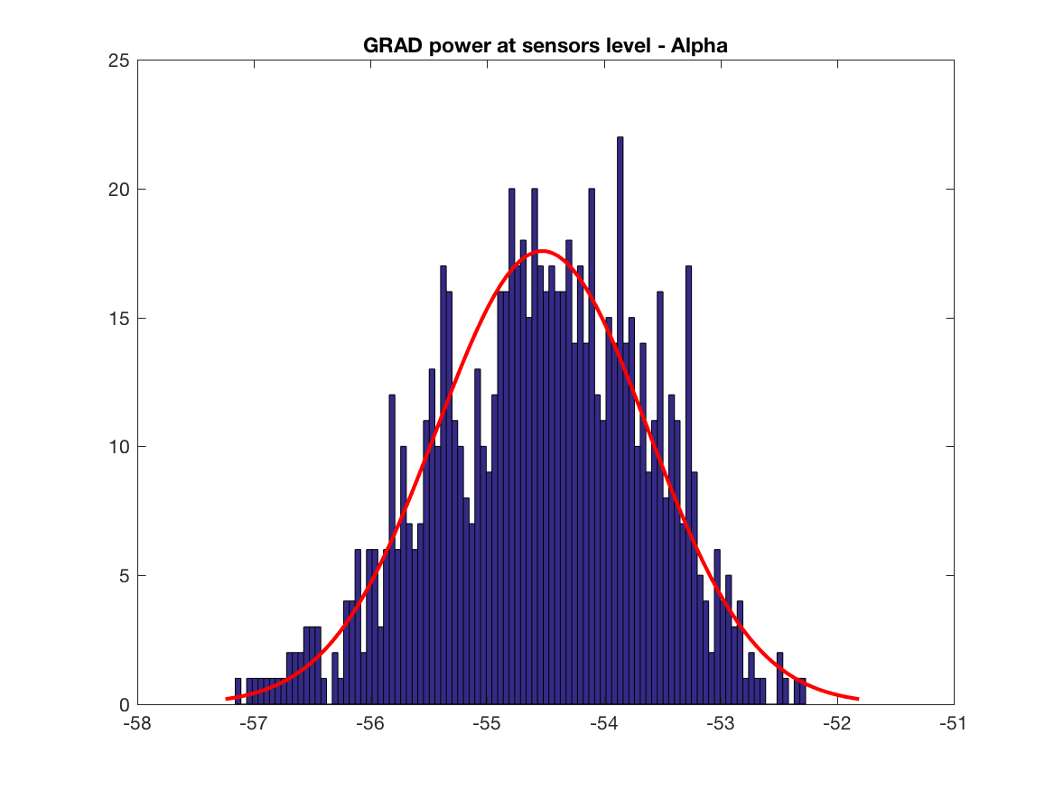
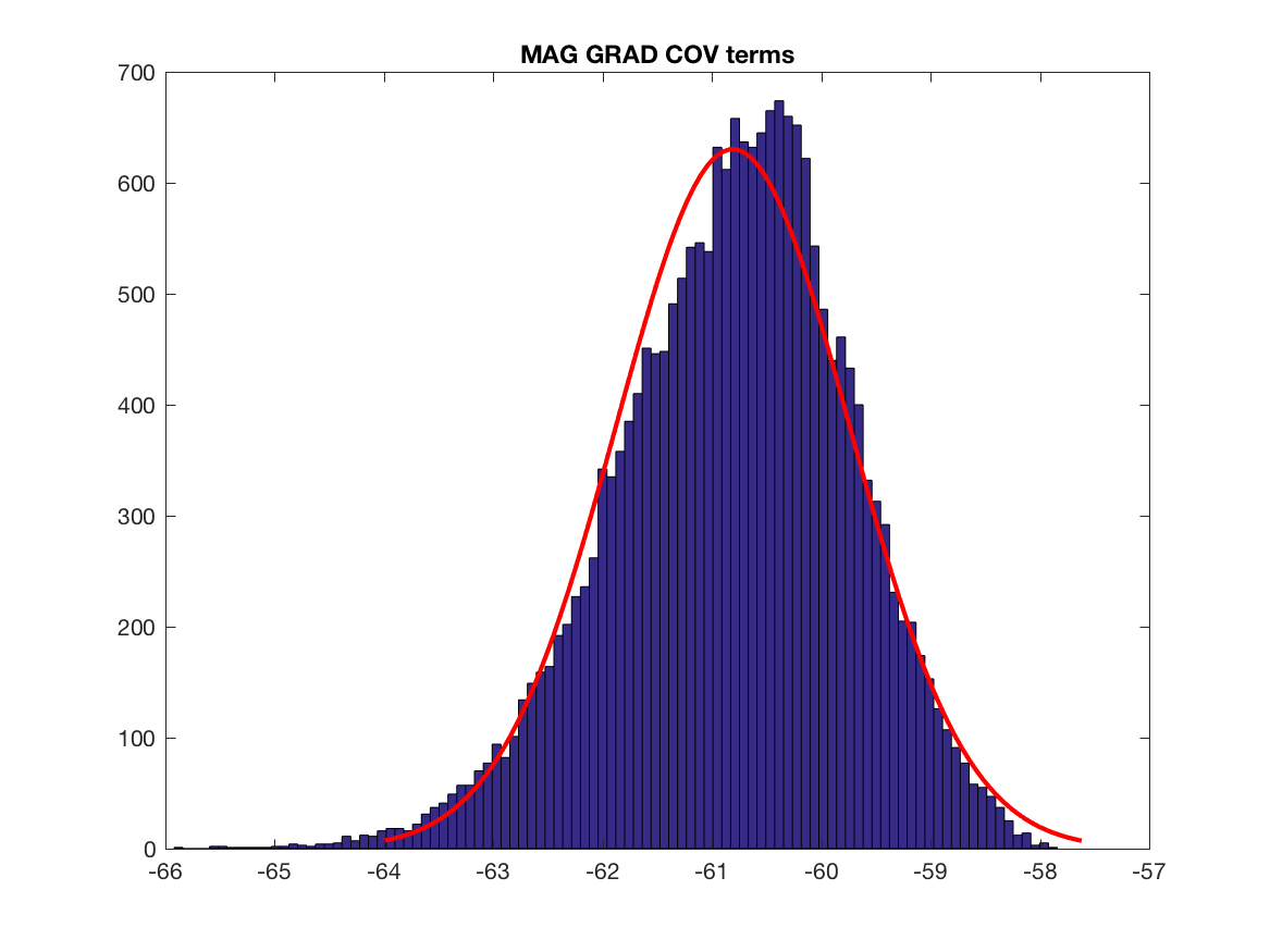
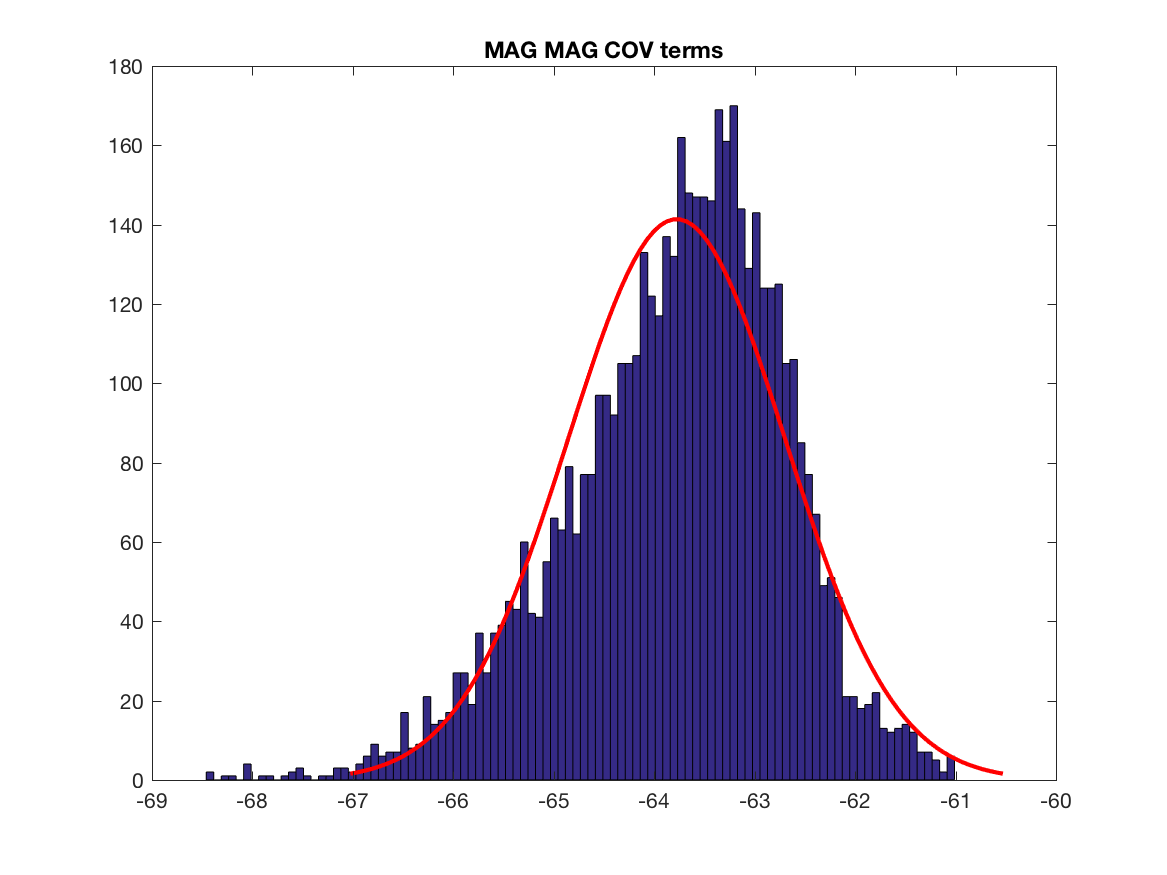
Let's dig a little bit further by analysing power of signals at sensors level and the corresponding content of the covariance matrix. We have to think about that point, difference in magnitude will play a role at one point. But the main point is the difference in the information content, i.e. the y axis of the histograms, we have much more covariance terms having GRAD data than MAG data, this may explain why we have mainly GRAD results in the localisation maps. Also this is one subject, we have to test other brain, sensors locations and do simulations (see below for the simulation).
%% Modified script for test combining MAG and GRAD with fieldtrip 051217 --- Based on Sarang Dalal sugestion
ft_defaults

[ trials ] = trial_definition_ft( {'cardiocor_blinkcor_run03_tsss.fif' 'cardiocor_blinkcor_run04_tsss.fif'}, 'LEFT_MVT_CLEAN', 2.0, 2.0, 'BIO005' ) ;

%% %% Basic configuration
overall_time_window = [-2 2] ; %% if you modify this modify the trials def above !

active_time_window = [0.2 0.6] ;

reference_time_window = [-1.4 -1.0] ;

beamformer_lambda_normalization = '10%' ;

lead_field_depth_normalization = 'column' ;

freqofinterest = 22 ;
freqhalfwin = 6 ;

load vol ; %% load head model located in the subject directory and obtained from the T1 MRI of the subject

load('mri_aligned.mat') ; %% MRI data needed for vizualisation
load('segmentedmri.mat') ;

% Select time window of interest
cfg = [];
cfg.toilim = active_time_window ;
data_timewindow_active = ft_redefinetrial(cfg,trials);
% Select time window of control
cfg = [];
cfg.toilim = reference_time_window ;
data_timewindow_ref = ft_redefinetrial(cfg,trials);
% Concatenate for common spatial filter
data_all = ft_appenddata([], data_timewindow_active, data_timewindow_ref);

channelsofinterest_meters = {'MEG'} ; %% Magnetometer on an Elekta system

%%%%%%%%%%%%%%%%%%%%%%%%%%%%%%%%%%%%%%%%%%%%%%%%%%%%%%%%%%%%%%%%%%%%%%%%%%
%% Analyse scale difference in power in the frequency of interest
%%%%%%%%%%%%%%%%%%%%%%%%%%%%%%%%%%%%%%%%%%%%%%%%%%%%%%%%%%%%%%%%%%%%%%%%%%

%% Time-frequency analysis of all the trials
cfg              = [];
cfg.output       = 'pow';
cfg.channel      = 'MEG';
cfg.method       = 'mtmconvol';
cfg.taper        = 'hanning';
cfg.foi          = 7:2:13;                         % analysis 2 to 30 Hz in steps of 2 Hz
cfg.t_ftimwin    = ones(length(cfg.foi),1).*0.5;   % length of time window = 0.5 sec
cfg.toi          = -2.0:0.05:2.0;                  % time window "slides" from -0.5 to 1.5 sec in steps of 0.05 sec (50 ms)
TFRchanneldata = ft_freqanalysis(cfg, trials);
title(['Time-Frequency Analysis']) ;

%% Average over time
TF_POW = mean(TFRchanneldata.powspctrm(:,:,30:50), 3) ;

%% Build on histrogram of MAG and GRAD values
[~, idxmag]= intersect(trials.label, ft_channelselection({'MEG*1'}, trials.label)) ;
[~, idxgrad]= intersect(trials.label, ft_channelselection({'MEG*2', 'MEG*3'}, trials.label)) ;

figure; histfit(log(reshape(TF_POW(idxmag,:),length(idxmag)*length(cfg.foi),1)),100)
title('MAG power at sensors level - Alpha')
print(['MAG_power_sensors_level_alpha'],'-dpng')
param_mag_sensors = fitdist(log(reshape(TF_POW(idxmag,:),length(idxmag)*length(cfg.foi),1)),'Normal') ;

figure; histfit(log(reshape(TF_POW(idxgrad,:),length(idxgrad)*length(cfg.foi),1)),100)
title('GRAD power at sensors level - Alpha')
print(['GRAD_power_sensors_level_alpha'],'-dpng')
param_grad_sensors = fitdist(log(reshape(TF_POW(idxgrad,:),length(idxgrad)*length(cfg.foi),1)),'Normal') ;

coef_norm_mag_sensors = exp(abs(param_grad_sensors.mu-param_mag_sensors.mu)) ;

for i_trial=1:length(data_all.trial)
    data_all.trial{1, i_trial}(idxmag,:) = data_all.trial{1, i_trial}(idxmag,:) * coef_norm_mag_sensors ;
end

for i_trial=1:length(data_timewindow_active.trial)
    data_timewindow_active.trial{1, i_trial}(idxmag,:) = data_timewindow_active.trial{1, i_trial}(idxmag,:) * coef_norm_mag_sensors ;
end

for i_trial=1:length(data_timewindow_ref.trial)
    data_timewindow_ref.trial{1, i_trial}(idxmag,:) = data_timewindow_ref.trial{1, i_trial}(idxmag,:) * coef_norm_mag_sensors ;
end

%%%%%%%%%%%%%%%%%%%%%%%%%%%%%%%%%%%%%%%%%%%%%%%%%%%%%%%%%%%%%%%%%%%%%%%%%%
%% DICS Analysis combining both gradiometers and magnetometers in meter %%
%%%%%%%%%%%%%%%%%%%%%%%%%%%%%%%%%%%%%%%%%%%%%%%%%%%%%%%%%%%%%%%%%%%%%%%%%%

%% Select MAG + GRAD sensors
channelsofinterest_meters = {'MEG'} ; %% Magnetometer on an Elekta system

powcsd_all = compute_crosprect(channelsofinterest_meters, freqofinterest, freqhalfwin, data_all) ;
powcsd_active = compute_crosprect(channelsofinterest_meters, freqofinterest, freqhalfwin, data_timewindow_active) ;
powcsd_ref = compute_crosprect(channelsofinterest_meters, freqofinterest, freqhalfwin, data_timewindow_ref) ;

range_of_weights = [1] ; %% 10 20 50 100 1000 10000 20000 50000 100000 200000 1e6] ;

roi_l = [2901 2649 2648 2662] ;
roi_r = [2909 3161 3175 2923] ;

res_left = zeros(length(roi_l), length(range_of_weights)) ;
res_right = zeros(length(roi_r), length(range_of_weights)) ;

idx_res = 1 ;

for i_weight=range_of_weights
    %% Convert the grad structure to meters (I do that in the cross spectrum matrix to speed the test, should be done at the very beginning on the data itself
    powcsd_all_meters = powcsd_all ;
    powcsd_active_meters = powcsd_active ;
    powcsd_ref_meters = powcsd_ref ;

    powcsd_all_meters.grad = ft_convert_units(powcsd_all.grad, 'm') ;
    powcsd_active_meters.grad = powcsd_all_meters.grad ;
    powcsd_ref_meters.grad = powcsd_all_meters.grad ;

    %% NO peculiar weighting for the MAG (Sarang way)
    wheigthing_coefficient = i_weight ;

    %% Convert the grad structure to meters (I do that in the cross spectrum matrix to speed the test, should be done at the very beginning on the data itself
    powcsd_all_meters = powcsd_all ;
    powcsd_active_meters = powcsd_active ;
    powcsd_ref_meters = powcsd_ref ;

    powcsd_all_meters.grad = ft_convert_units(powcsd_all.grad, 'm') ;
    powcsd_active_meters.grad = powcsd_all_meters.grad ;
    powcsd_ref_meters.grad = powcsd_all_meters.grad ;

    grad_grad = [] ;
    index_grad_grad = 1 ;

    mag_mag = [] ;
    index_mag_mag = 1 ;

    mag_grad = [] ;
    index_mag_grad = 1 ;

    %% Lets analyse the covariance matrix
    for (i_dipole=1:length(powcsd_active_meters.labelcmb))
        if powcsd_active.labelcmb{i_dipole,1}(end) == '1' %% its a mag
            if powcsd_active.labelcmb{i_dipole,2}(end) == '2' || powcsd_active.labelcmb{i_dipole,2}(end) == '3' %% its a grad
                mag_grad(index_mag_grad) = powcsd_all.crsspctrm(i_dipole) ; index_mag_grad = index_mag_grad + 1 ;
            else
                mag_mag(index_mag_mag) = powcsd_all.crsspctrm(i_dipole) ; index_mag_mag = index_mag_mag + 1 ;
            end
        else %% its a grad
            if powcsd_active.labelcmb{i_dipole,2}(end) == '1' %% its a mag
                mag_grad(index_mag_grad) = powcsd_all.crsspctrm(i_dipole) ; index_mag_grad = index_mag_grad + 1 ;
            else
                grad_grad(index_grad_grad) = powcsd_all.crsspctrm(i_dipole) ; index_grad_grad = index_grad_grad + 1 ;
            end
        end
    end

    figure; histfit(log(abs(grad_grad)),100)
    title('GRAD GRAD COV terms')
    print(['GRAD_GRAD_COV_terms'],'-dpng')
    param_grad_grad = fitdist(log(abs(grad_grad))','Normal') ;

    figure; histfit(log(abs(mag_grad)),100)
    title('MAG GRAD COV terms')
    print(['MAG_GRAD_COV_terms'],'-dpng')
    param_mag_grad = fitdist(log(abs(mag_grad))','Normal') ;

    coef_norm_mag_grad = exp(abs(param_grad_grad.mu-param_mag_grad.mu)) ;
    %%coef_norm_mag_grad = 0.0 ;

    figure; histfit(log(abs(mag_mag)),100)
    title('MAG MAG COV terms')
    print(['MAG_MAG_COV_terms'],'-dpng')
    param_mag_mag = fitdist(log(abs(mag_mag))','Normal') ;

    coef_norm_mag_mag = exp(abs(param_grad_grad.mu-param_mag_mag.mu)) ;

    %% Lets tripote the covariance matrix (with the help of Sarang) - I put to zeros all the crossterms between mag and grad
    for (i_dipole=1:length(powcsd_active_meters.labelcmb))
        if powcsd_active.labelcmb{i_dipole,1}(end) == '1' %% its a mag
            if powcsd_active.labelcmb{i_dipole,2}(end) == '2' || powcsd_active.labelcmb{i_dipole,2}(end) == '3' %% its a grad
                powcsd_all_meters.crsspctrm(i_dipole) = powcsd_all_meters.crsspctrm(i_dipole) * coef_norm_mag_grad ;
                powcsd_active_meters.crsspctrm(i_dipole) = powcsd_active_meters.crsspctrm(i_dipole) * coef_norm_mag_grad ;
                powcsd_ref_meters.crsspctrm(i_dipole) = powcsd_ref_meters.crsspctrm(i_dipole) * coef_norm_mag_grad ;
            else
                powcsd_all_meters.crsspctrm(i_dipole) = powcsd_all_meters.crsspctrm(i_dipole) * coef_norm_mag_mag ;
                powcsd_active_meters.crsspctrm(i_dipole) = powcsd_active_meters.crsspctrm(i_dipole) * coef_norm_mag_mag ;
                powcsd_ref_meters.crsspctrm(i_dipole) = powcsd_ref_meters.crsspctrm(i_dipole) * coef_norm_mag_mag ;
            end
        else %% its a grad
            if powcsd_active.labelcmb{i_dipole,2}(end) == '1' %% its a mag
                powcsd_all_meters.crsspctrm(i_dipole) = powcsd_all_meters.crsspctrm(i_dipole) * coef_norm_mag_grad ;
                powcsd_active_meters.crsspctrm(i_dipole) = powcsd_active_meters.crsspctrm(i_dipole) * coef_norm_mag_grad ;
                powcsd_ref_meters.crsspctrm(i_dipole) = powcsd_ref_meters.crsspctrm(i_dipole) * coef_norm_mag_grad ;
            end
        end
    end

    %% In complement and for coherence lets also adapt the variance of each mag accordingly
    [~, idxmag]= intersect(trials.label, ft_channelselection({'MEG*1'}, trials.label)) ;
    powcsd_all_meters.powspctrm(idxmag) = powcsd_all_meters.powspctrm(idxmag) * coef_norm_mag_mag ;
    powcsd_active_meters.powspctrm(idxmag) = powcsd_active_meters.powspctrm(idxmag) * coef_norm_mag_mag ;
    powcsd_ref_meters.powspctrm(idxmag) = powcsd_ref_meters.powspctrm(idxmag) * coef_norm_mag_mag ;

    % Create leadfield grid
    cfg                 = [];
    cfg.channel         = channelsofinterest_meters ;
    cfg.grad            = powcsd_active_meters.grad;
    cfg.vol             = vol ;
    cfg.dics.reducerank = 2; % default for MEG is 2, for EEG is 3
    cfg.grid.resolution = 0.01;   % use a 3-D grid with a 0.5 cm resolution %% I sippose this should be in meter now ...
    cfg.grid.unit       = 'm';
    cfg.grid.tight      = 'yes';
    cfg.normalize       =  lead_field_depth_normalization ; %% Depth normalization
    [grid_meters] = ft_prepare_leadfield(cfg);


    %% %%%%%%%%%% DICS %%%%%%%%%%

    %% Compute DICS filters for the concatenated data
    cfg              = [];
    cfg.channel      = channelsofinterest_meters ;
    cfg.method       = 'dics';
    cfg.frequency    = freqofinterest ;
    cfg.grid         = grid_meters;
    cfg.headmodel    = vol;
    cfg.senstype     = 'MEG'; % Must me 'MEG', although we only kept MEG channels, information on EEG channels is still present in data
    cfg.dics.keepfilter   = 'yes'; % We wish to use the calculated filter later on
    cfg.dics.projectnoise = 'yes';
    cfg.dics.lambda  = beamformer_lambda_normalization;
    source_all_meters = ft_sourceanalysis(cfg, powcsd_all_meters);

    %% Apply computed filters to each active and reference windows
    cfg              = [];
    cfg.channel      = channelsofinterest_meters ;
    cfg.method       = 'dics';
    cfg.frequency    = freqofinterest ;
    cfg.grid         = grid_meters;
    cfg.grid.filter  = source_all_meters.avg.filter;
    cfg.dics.projectnoise = 'yes';
    cfg.headmodel          = vol;
    cfg.dics.lambda  = beamformer_lambda_normalization ;
    cfg.senstype     ='MEG' ;

    %% Source analysis active
    source_active_meters = ft_sourceanalysis(cfg, powcsd_active_meters);

    %% Source analysis reference
    source_reference_meters = ft_sourceanalysis(cfg, powcsd_ref_meters);

    %% Compute differences (power) between active and reference
    source_diff_meters = source_active_meters ;
    source_diff_meters.avg.pow  = (source_active_meters.avg.pow - source_reference_meters.avg.pow) ./ (source_active_meters.avg.pow + source_reference_meters.avg.pow);

    %% Store the results in roi for later analysis
    for idx_roi=1:length(roi_l)
        res_left(idx_res,idx_roi)=source_diff_meters.avg.pow(roi_l(idx_roi));
    end
    for idx_roi=1:length(roi_r)
        res_right(idx_res,idx_roi)=source_diff_meters.avg.pow(roi_r(idx_roi));
    end
    idx_res = idx_res + 1 ;

    %% Display the results
    visuBF( source_diff_meters, 'title' )
    title(['Combining MAG+GRAD - dalal way with adapted coef']) ;
    print(['comb_mag_grad_dalal-adapted'],'-dpng')
end

%% Without scaling of the cross modality covariance
%% With full scaling, clearly it does not work
We will do some simulation to explore in detail the following points:
- Effect of noise on beamformer results with respect to: source depth and kind of sensors
- Effect of the MAG and GRAD mixing using the different ways tested above
Simulation setup:
- We use the sensors configuration from subject1 (see above)
ft_defaults

%% Lets seed the random number generator (seed based on current time)
rng('shuffle') ;
%% Load real signals and grid (sensors location, grid points, trials struct)
[ trials ] = trial_definition_ft( {'cardiocor_blinkcor_run03_tsss.fif' 'cardiocor_blinkcor_run04_tsss.fif'}, 'LEFT_MVT_CLEAN', 2.0, 2.0, 'BIO005' ) ;

%% Basic configuration
overall_time_window = [-2 2] ; %% if you modify this modify the trials def above !

active_time_window = [0.2 0.6] ;
reference_time_window = [-1.4 -1.0] ;
beamformer_lambda_normalization = '10%' ;

lead_field_depth_normalization = 'column' ;

freqofinterest = 22 ;
freqhalfwin = 6 ;

load vol ; %% for the grid

%% load('mri_aligned.mat') ; %% MRI data needed for visualisation
%% load('segmentedmri.mat') ;

%% convert sensors location in meter
grad_meters = ft_convert_units(trials.grad, 'm') ;

% Create temporary lead field for the simulation
cfg                 = [];
cfg.channel         = 'MEG' ;
cfg.grad            = grad_meters ;
cfg.vol             = vol ;
cfg.dics.reducerank = 2; % default for MEG is 2, for EEG is 3
cfg.grid.resolution = 0.01;   % use a 3-D grid with a 0.5 cm resolution %% I sippose this should be in meter now ...
cfg.grid.unit       = 'm';
cfg.grid.tight      = 'yes';
cfg.normalize       =  lead_field_depth_normalization ; %% Depth normalization
[grid_meters_simu] = ft_prepare_leadfield(cfg);

%% Get the indexes of grid points inside the brain
[I]=find(grid_meters_simu.inside)

%% Compute the lead field to used during the localisation (i.e. with the sensors configuration we want to test)


%% %% Select MAG or GRAD or MAG & GRAD sensors
channelsofinterest_meters = {'MEG*1'} ; %% Magnetometer on an Elekta system
%% channelsofinterest_meters = {'MEG*2', 'MEG*3'};

% Create leadfield grid
cfg                 = [];
cfg.channel         = channelsofinterest_meters ;
cfg.grad            = grad_meters ;
cfg.vol             = vol ;
cfg.dics.reducerank = 2; % default for MEG is 2, for EEG is 3
cfg.grid.resolution = 0.01;   % use a 3-D grid with a 0.5 cm resolution %% I sippose this should be in meter now ...
cfg.grid.unit       = 'm';
cfg.grid.tight      = 'yes';
cfg.normalize       =  lead_field_depth_normalization ; %% Depth normalization
[grid_meters] = ft_prepare_leadfield(cfg);
- We defined two sources one "cortical", another one 'deep'
- Simulated activity is the sum of the recurrent activity of the fixed source with an oscillating activity around 22Hz between 2 and 4 s and the activity of a randomly chosen source with an oscillating time course between 0 and 50 Hz between -2 to 2 s. The randomly chosen source changes at each trial. The whole process is repeated to derive variability measure.
%% Source activity
noise_scale = noise_level ;
phase_scale = 10 ;
frequency = 22 ;
x = 0:0.001:3.999 ;
%% Chosen grid point, for one simulations set we use only one
cortex_id = 3381 ;
deep_id = 1621 ;
grid_meters_simu.leadfield{deep_id}
leadfield=grid_meters_simu.leadfield{deep_id};
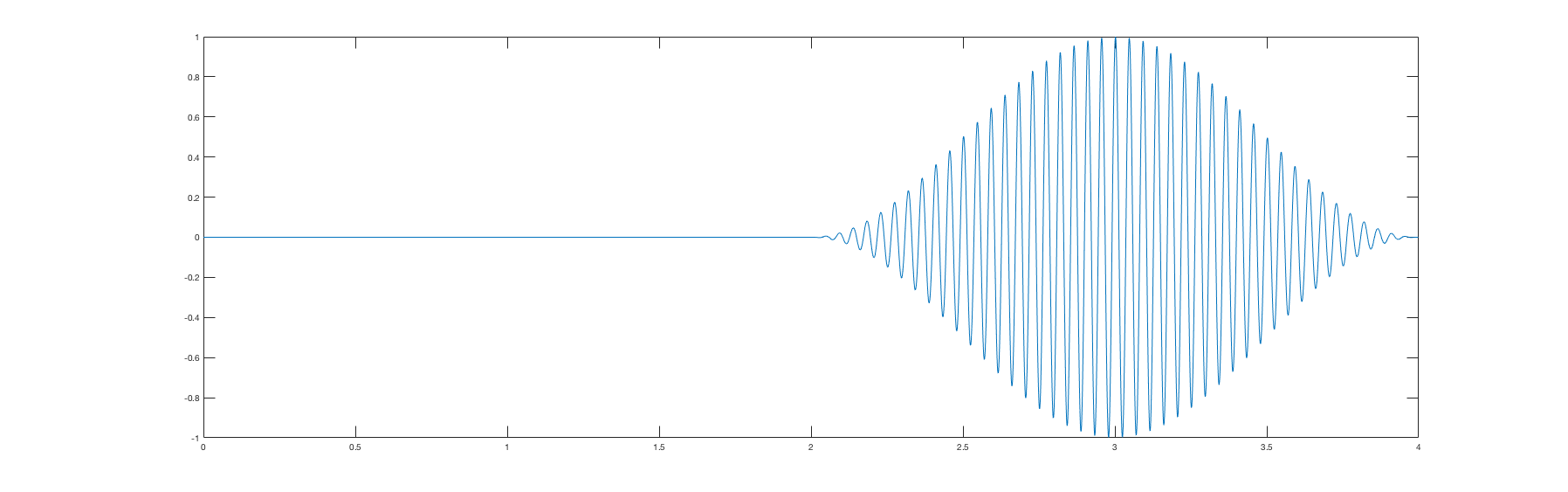
%% Source time course and corresponding sensors level signals - no noise here except a slight phase shift (i.e. we consider intrinsic sensor noise negligible. First half of the time window: no source activity, second half: windowed oscillation at the chosen frequency. We recompute the activity for each trial (phase shift will be use later to explore connectivity)
for i_trial=1:length(trials.trialinfo)
phase_shift = rand(1,1)*phase_scale ;
activity= sin(frequency*2*3.14116*(x+phase_shift)).* [zeros(1,length(x)/2) hann(length(x)/2)'];
sensors=leadfield*[1 0 0]'*activity; %% source has a tangential orientation
trials.trial{i_trial}(1:306,:)=sensors ;
end
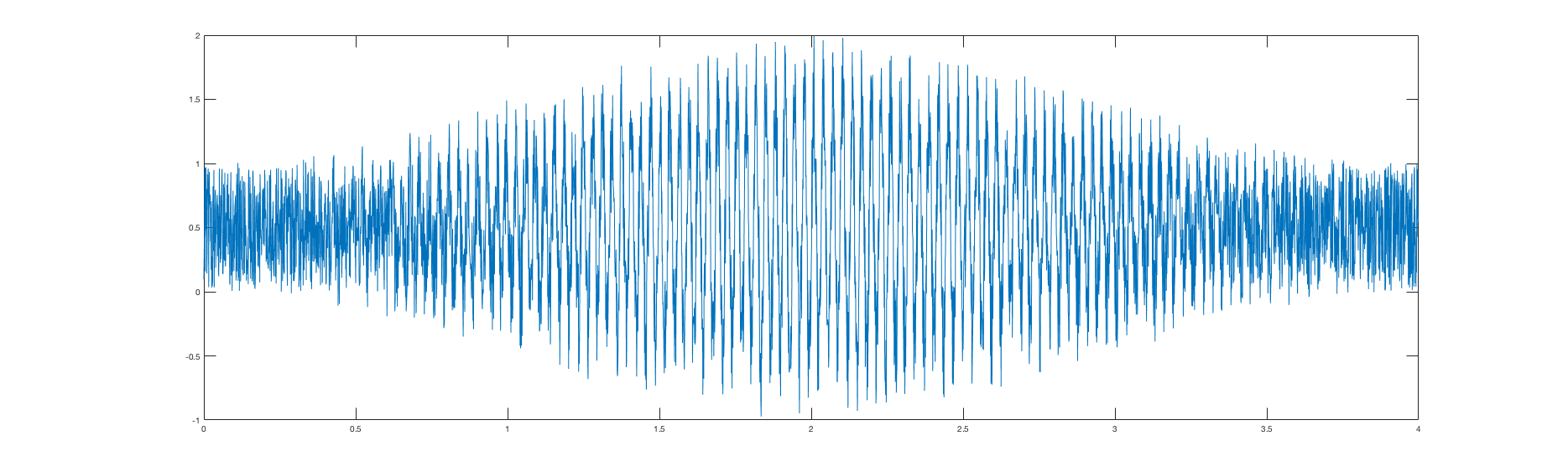
%% Noise: noise comes from random sources activity. We choose (randomly) a grid point for each trial and source time course is a constant oscillation at a random frequency (0 to 50 Hz) plus white noise (the whole thing is windowed at the extremity of the time window. The corresponding sensors level signal is added to the signal computed above
for i_trial=1:length(trials.trialinfo)
phase_shift = rand(1,1)*phase_scale ;
activity= sin(rand(1,1)*50*2*3.14116*(x+phase_shift)).* [hann(length(x))']+rand(1,length(x))*noise_scale; %% Noise scale intervenes here
index_source = ceil(rand(1,1)*(length(I))) ;
leadfield=grid_meters_simu.leadfield{I(index_source)};
sensors=leadfield*[1 0 0]'*activity;
trials.trial{i_trial}(1:306,:)=trials.trial{i_trial}(1:306,:)+sensors; %% We add activity coming from the fixed source and the random scaled with the noise level
end
% Select time window of interest
cfg = [];
cfg.toilim = active_time_window ;
data_timewindow_active = ft_redefinetrial(cfg,trials);
% Select time window of control
cfg = [];
cfg.toilim = reference_time_window ;
data_timewindow_ref = ft_redefinetrial(cfg,trials);
% Concatenate for common spatial filter
data_all = ft_appenddata([], data_timewindow_active, data_timewindow_ref);
Localisation step:
 		% Select time window of interest
        cfg = [];
        cfg.toilim = active_time_window ;
        data_timewindow_active = ft_redefinetrial(cfg,trials);
        % Select time window of control
        cfg = [];
        cfg.toilim = reference_time_window ;
        data_timewindow_ref = ft_redefinetrial(cfg,trials);
        % Concatenate for common spatial filter
        data_all = ft_appenddata([], data_timewindow_active, data_timewindow_ref);

        %%%%%%%%%%%%%%%%%%%%%%%%%%%%%%%%%%%%%%%%%%%%%%%%%%%%%%%%%%%%%%%%%%%%%%%%%%
        %% DICS Analysis combining both gradiometers and magnetometers in meter %%
        %%%%%%%%%%%%%%%%%%%%%%%%%%%%%%%%%%%%%%%%%%%%%%%%%%%%%%%%%%%%%%%%%%%%%%%%%%
        powcsd_all = compute_crosprect(channelsofinterest_meters, freqofinterest, freqhalfwin, data_all) ;
        powcsd_active = compute_crosprect(channelsofinterest_meters, freqofinterest, freqhalfwin, data_timewindow_active) ;
        powcsd_ref = compute_crosprect(channelsofinterest_meters, freqofinterest, freqhalfwin, data_timewindow_ref) ;

        %% Convert the grad structure to meters (I do that in the cross spectrum matrix to speed the test, should be done at the very beginning on the data itself

        powcsd_all_meters = powcsd_all ;
        powcsd_active_meters = powcsd_active ;
        powcsd_ref_meters = powcsd_ref ;

        powcsd_all_meters.grad = ft_convert_units(powcsd_all.grad, 'm') ;
        powcsd_active_meters.grad = powcsd_all_meters.grad ;
        powcsd_ref_meters.grad = powcsd_all_meters.grad ;

        %% %%%%%%%%%% DICS %%%%%%%%%%
        %% Compute DICS filters for the concatenated data

        cfg              = [];
        cfg.channel      = channelsofinterest_meters ;
        cfg.method       = 'dics';
        cfg.frequency    = freqofinterest ;
        cfg.grid.pos           = grid_meters.pos(cortex_id,:) ;
        cfg.grid.inside        = 1 ;
        cfg.grid.outside       = [] ;
        cfg.grid.unit         = 'm' ;
        cfg.headmodel    = vol;
        cfg.senstype     = 'MEG'; % Must me 'MEG', although we only kept MEG channels, information on EEG channels is still present in data
        cfg.dics.keepfilter   = 'yes'; % We wish to use the calculated filter later on
        cfg.dics.projectnoise = 'yes';
        cfg.dics.lambda  = beamformer_lambda_normalization;
        source_all_meters = ft_sourceanalysis(cfg, powcsd_all_meters);

        %% Apply computed filters to each active and reference windows
        cfg              = [];
        cfg.channel      = channelsofinterest_meters ;
        cfg.method       = 'dics';
        cfg.frequency    = freqofinterest ;
        cfg.grid.pos           = grid_meters.pos(cortex_id,:) ;
        cfg.grid.inside        = 1 ;
        cfg.grid.outside       = [] ;
        cfg.grid.unit         = 'm' ;
        cfg.headmodel    = vol;
        cfg.grid.filter  = source_all_meters.avg.filter;
        cfg.dics.projectnoise = 'yes';
        cfg.headmodel          = vol;
        cfg.dics.lambda  = beamformer_lambda_normalization ;
        cfg.senstype     ='MEG' ;

        %% Source analysis active
        source_active_meters = ft_sourceanalysis(cfg, powcsd_active_meters);

        %% Source analysis reference
        source_reference_meters = ft_sourceanalysis(cfg, powcsd_ref_meters);

        %% Compute differences (power) between active and reference
        source_diff_meters = source_active_meters ;

        source_diff_meters.avg.pow  = (source_active_meters.avg.pow - source_reference_meters.avg.pow) ./ (source_active_meters.avg.pow + source_reference_meters.avg.pow);

        diff_act(idx_repet, idx_res) = source_diff_meters.avg.pow(1) ;
- noise
Sources activity
Random sources activity
First simulation results - will be modified
Results with MAG
At source location :
At another location (quite far) :
We will use that to threshold the simulated data
Do the same for GRAD
Do the same with MAG + GRAD (all approaches)