This is a collaborative space. In order to contribute, send an email to maximilien.chaumon@icm-institute.org
On any page, type the letter L on your keyboard to add a "Label" to the page, which will make search easier.
Single trials - Connectivity analysis - Cortico-muscular coherency
In this tutorial, you will find a description of all the steps necessary to obtain a virtual sensor time course using a LCMV beamformer approach in FieldTrip for one subject.
Prerequisites
- Read the previous tutorials (MEG EEG pre-processing, MEG sensors realignment, filter, baseline correction)
- Pre process the T1 MRI data or choose a template
- Download the latest version of FieldTrip - Install it in your software folder - Take a look at the FieldTrip tutorials!
Input data
MEG signals (MEG)
FieldTrip can import the fif files coming from our MEG system and those pre processed with our in-house tools. If you acquired simultaneous MEG+EEG data, FieldTrip will import both of them.
MRI
If you have the individual anatomy of each of your subjects (T1 MRI), you should process it with FieldTrip as described below.
If you don't have the individual anatomy, then you have to choose a template in FieldTrip.
Needed software
For MEG fif files pre processed outside FieldTrip: You will need two in-house scripts to read the marker files we add to the MEG fif files (put them in your matlab path):
A short script to pre process the MRI in FieldTrip: pre_process_mri_for_ft.m
A simple script to visualize beamformer results: visuBF.m
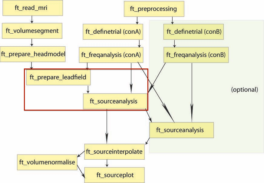
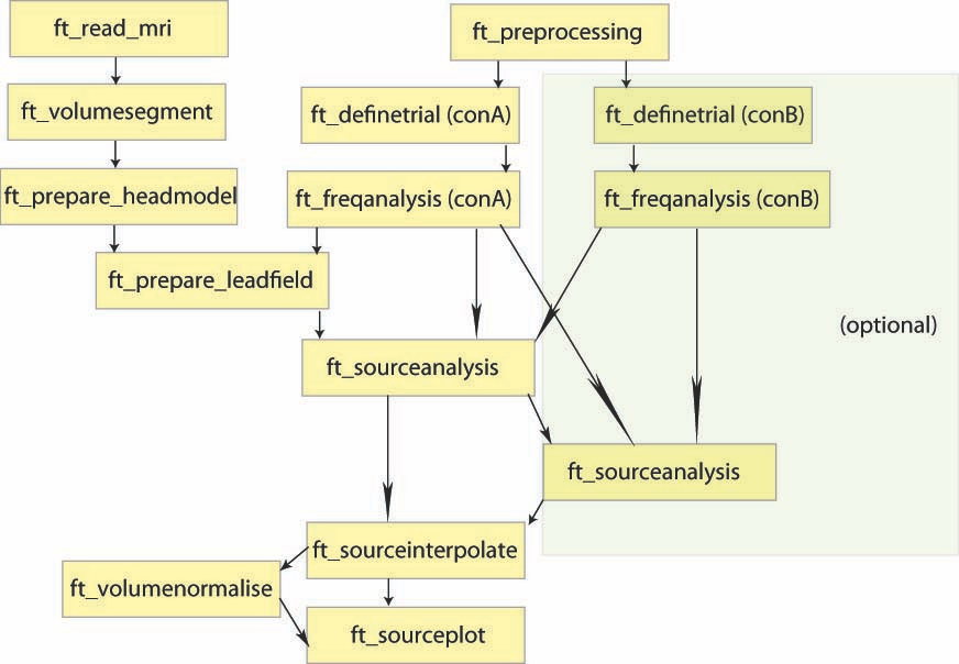
LCMV analysis with FieldTrip
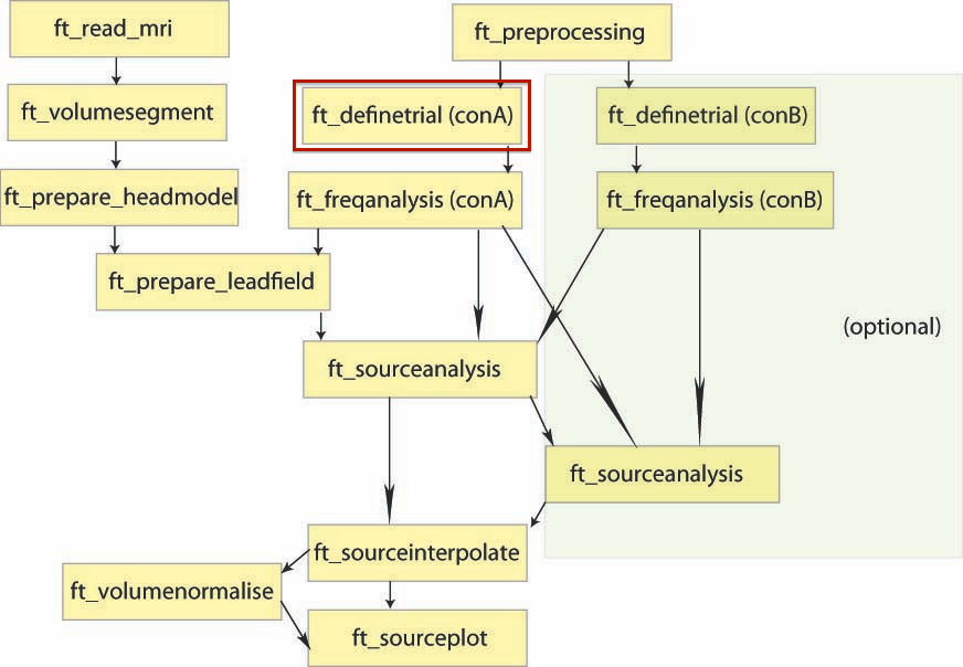
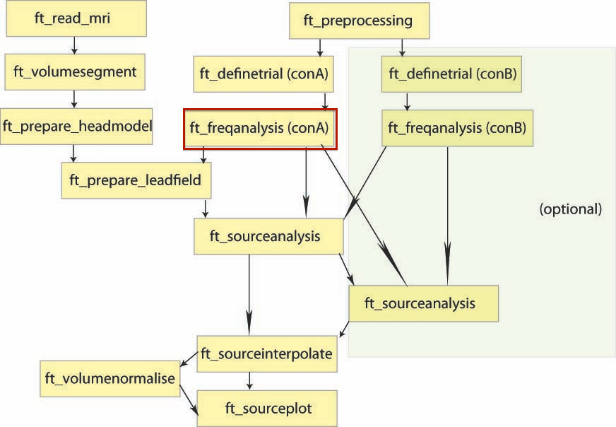
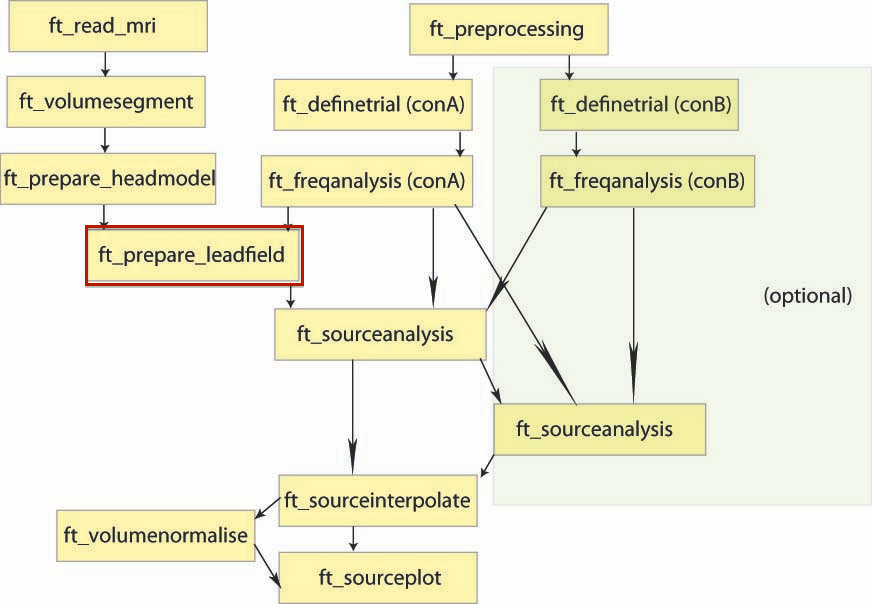
Overview of the process:
Suggested data organisation
The mat files generated by FieldTrip can be stored together with the pre-processed data. You may want to create a specific sub folder "FT" to store them in each subject.
Read data
The data should be pre processed (i.e. artefact free) at this point and the FieldTrip folder in your matlab path.
ft_defaults ; %% Load fieldtrip configuration

%% Read two runs, define trials around LEFT_MVT_CLEAN marker (-2s to 2s around the marker), read also BIO005 which is an EMG.
[ trials ] = trial_definition_ft( {'cardiocor_blinkcor_run03_tsss.fif' 'cardiocor_blinkcor_run04_tsss.fif'}, 'LEFT_MVT_CLEAN', 2.0, 2.0, 'BIO005' ) ;
Covariance Computation
%% Compute covariance of the data (as a whole - both conditions)
cfg                   = [];
cfg.covariance        = 'yes';
cfg.channel           = channelsofinterest ;
cfg.vartrllength      = 0;
cfg.covariancewindow  = 'all';
cfg.trials            = 'all';
tlock                 = ft_timelockanalysis(cfg, trials);
Forward operator
We compute the leans field based on the warped MNI grid.
% Create leadfield grid

cfg                 = [];
cfg.channel         = channelsofinterest ;
cfg.grad            = data_all.grad;
cfg.vol             = vol ;
cfg.dics.reducerank = 2; % default for MEG is 2, for EEG is 3
cfg.grid.resolution = 1.0;   % use a 3-D grid with a 0.5 cm resolution
cfg.grid.unit       = 'cm';
cfg.grid.tight      = 'yes';
cfg.normalize       =  lead_field_depth_normalization ; %% Depth normalization
[grid] = ft_prepare_leadfield(cfg);
LCMV Analysis
The spatial filters are computed here. We then contrast the two conditions before saving the results.
%% LCMV ANALYSIS TO GET TEMPORAL INFORMATION with virtual sensors
%% Retrieve correct labelling of the trials
data_all.trialinfo = [zeros(length(data_timewindow_active.trial), 1); ones(length(data_timewindow_ref.trial), 1)];
%% Compute covariance of the data (as a whole - both conditions)
cfg = [];
cfg.covariance = 'yes';
cfg.channel = channelsofinterest ;
cfg.vartrllength = 0;
cfg.covariancewindow = 'all';
cfg.trials = 'all';
tlock = ft_timelockanalysis(cfg, trials);
%% Let's choose a location of interest, here the central cursus we will define our virtual channels based on this seed WARNING: Unit = centimetre
pos_cm = [4.0 2.0 10.0 ] ;
%% Used to store the EP computed at each virtual sensor location
evoked_virtual_zscore = {} ;
evoked_virtual = {} ;
%% Compute filter for corresponding virtual sensor
cfg = [];
cfg.method = 'lcmv';
cfg.headmodel = vol ;
cfg.grid.pos = pos_cm ;
cfg.grid.inside = 1:size(cfg.grid.pos, 1);
cfg.grid.outside = [];
cfg.grid.unit = 'cm'; %% DO NOT FORGET THAT !
cfg.keepfilter = 'yes';
cfg.lcmv.fixedori = 'yes'; % project on axis of most variance using SVD
cfg.lcmv.projectnoise = 'yes' ;
cfg.lcmv.lambda = beamformer_lambda_normalization ;
cfg.lcmv.weightnorm = 'nai' ;
cfg.lcmv.normalize = lead_field_depth_normalization ; %% Depth normalization
source_idx = ft_sourceanalysis(cfg, tlock);
beamformer = source_idx.avg.filter{1};
%% Apply filter to the raw data
chansel = ft_channelselection(channelsofinterest, data_all.label); % find MEG sensor names
chansel = match_str(data_all.label, chansel);
virtualchanneldata = [];
virtualchanneldata.label = {'virtual_sensor'};
virtualchanneldata.time = trials.time;
for i=1:length(trials.trial)
virtualchanneldata.trial{i} = beamformer * trials.trial{i}(chansel,:);
end
%% Time-frequency analysis
cfg = [];
cfg.output = 'pow';
cfg.channel = 'virtual_sensor';
cfg.method = 'mtmconvol';
cfg.taper = 'hanning';
cfg.foi = 7:2:40; % analysis 2 to 40 Hz in steps of 2 Hz
cfg.t_ftimwin = ones(length(cfg.foi),1).*0.5; % length of time window = 0.5 sec
cfg.toi = -2.0:0.05:2.0; % time window "slides" from -0.5 to 1.5 sec in steps of 0.05 sec (50 ms)
TFRvirtualchanneldata = ft_freqanalysis(cfg, virtualchanneldata);
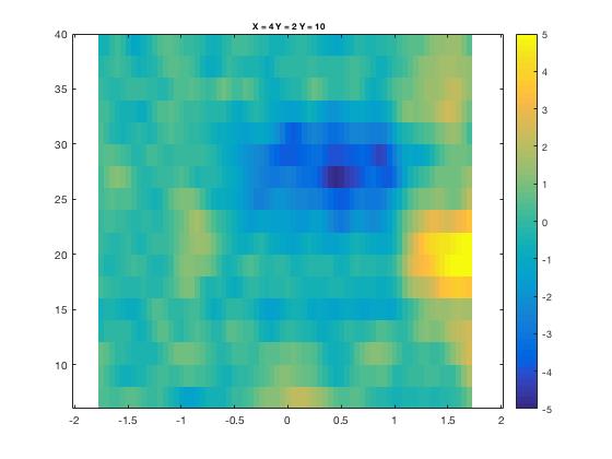
%% Display the results as a TF map
cfg = [];
cfg.baseline = reference_time_window ;
cfg.baselinetype = 'db';
cfg.channelname = 'virtual_sensor'; % top figure
cfg.zlim = [-5 5] ;
figure;ft_singleplotTFR(cfg, TFRvirtualchanneldata);
title(['X = ' num2str(pos_cm(1)) ' Y = ' num2str(pos_cm(2)) ' Y = ' num2str(pos_cm(3))]) ;
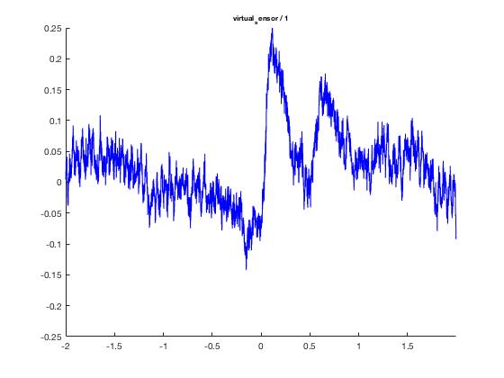
%% Evoked potential on the virtual sensor
cfg.demean = 'yes';
cfg.baselinewindow = reference_time_window;
evoked_virtual{1} = ft_timelockanalysis(cfg, virtualchanneldata);
%% Display the evoked potential
cfg.ylim = [-0.25 0.25] ;
figure ; ft_singleplotER(cfg, evoked_virtual{1}) ;