This is a collaborative space. In order to contribute, send an email to maximilien.chaumon@icm-institute.org
On any page, type the letter L on your keyboard to add a "Label" to the page, which will make search easier.
Mapping HCP MEG sources to an atlas
Prerequisite
HCP data has been unzipped to a local folder. The required files are
1. labelled anatomy files from the structural data processing pipeline, found in the ######_3T_Structural_preproc.zip files.
######/MNINonLinear/Native/######.L.aparc.a2009s.native.label.gii
######/MNINonLinear/Native/######.R.aparc.a2009s.native.label.gii
######/T1w/Native/######.L.midthickness.native.surf.gii
######/T1w/Native/######.L.midthickness.native.surf.gii
2. Left and right hemisphere surface source spaces as well as transformations from the MEG anatomy pipeline, found in files ######_MEG_anatomy.zip
######/MEG/anatomy/######.L.midthickness.4k_fs_LR.surf.gii
######/MEG/anatomy/######.R.midthickness.4k_fs_LR.surf.gii
######/MEG/anatomy/######.MEG_anatomy_transform.txt
3. the unzipped MEGconnectome pipeline megconnectome-3.0.zip (do not download the recommended version of FieldTrip if you are using a recent MATLAB (I tested with 2017b) because the syntax of MATLAB has slightly changed and FieldTrip won't run on your computer).
Goal of this tutorial
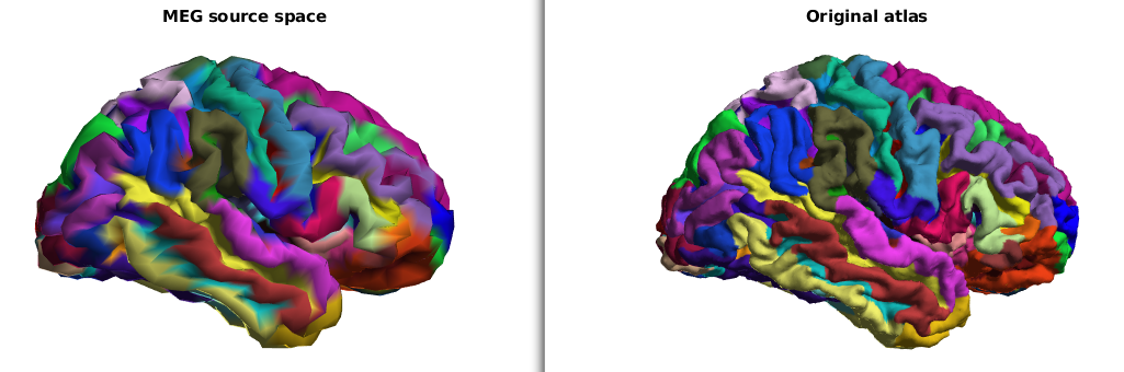
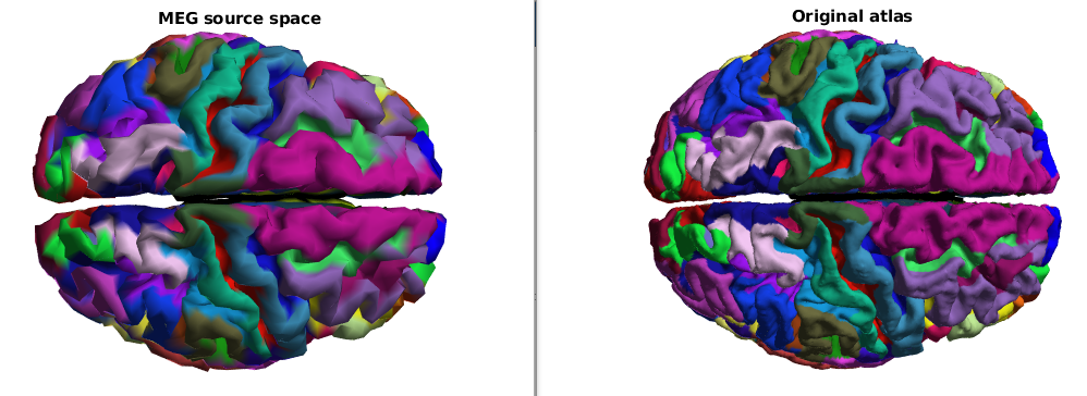
This tutorial describes a way to obtain anatomically labelled sources with HCP data.
Step-by-step guide
- Read labels and high definition structural data
- Read 2 hemisphere source spaces
- Combine them to get a labelled source space
- Plot the results
% add FieldTrip and the megconnectome folders to the path
addpath('/path/to/your/FieldTrip')
addpath(genpath('/path/to/your/megconnectome-3.0/'))% genpath includes subdirectories

Lsurf_fname = '/path/to/######/MEG/anatomy/######.L.midthickness.4k_fs_LR.surf.gii';
Rsurf_fname = '/path/to/######/MEG/anatomy/######.R.midthickness.4k_fs_LR.surf.gii';
transform_fname = '/path/to/######/MEG/anatomy/######.MEG_anatomy_transform.txt';
labs_fname = {'/path/to/######/MNINonLinear/Native/######.L.aparc.a2009s.native.label.gii',
			  '/path/to/######/MNINonLinear/Native/######.R.aparc.a2009s.native.label.gii'};
geoms_fname = {'/path/to/######/T1w/Native/######.L.midthickness.native.surf.gii',
			   '/path/to/######/T1w/Native/######.R.midthickness.native.surf.gii'};

% Read both hemispheres source spaces
Lsurf=ft_read_headshape(Lsurf_fname);
Rsurf=ft_read_headshape(Rsurf_fname);

% Read transforms
tmp = hcp_read_ascii(transform_fname);
transform = tmp.transform; clear tmp;

% merge them in one structure
ctxsm=Lsurf;
ctxsm.pos=[Lsurf.pos ;Rsurf.pos];
ctxsm.tri=[Lsurf.tri ; Rsurf.tri + size(Rsurf.pos,1)];

% convert to mm units and change the coordinate system (transforms are in mm)
ctxsm = ft_convert_units(ctxsm, 'mm');
ctxsm = ft_transform_geometry(transform.spm2bti, ctxsm);

% read atlas
labels = hcp_read_atlas(labs_fname);
geoms = ft_read_headshape({geoms_fname});

atlas = hcp_mergestruct(labels,geoms);
atlas.rgba = [atlas.rgba(:,1:3);atlas.rgba(:,1:3)];
atlas.unit = 'mm';

atlas = ft_transform_geometry(transform.spm2bti, atlas);

cfg = [];
cfg.interpmethod = 'nearest';
cfg.parameter = 'parcellation';
tmp = ft_sourceinterpolate(cfg,atlas,ctxsm);

ctxsm.parcellation = tmp.parcellation;
ctxsm.parcellationlabel = atlas.parcellationlabel;
ctxsm.rgba = [atlas.rgba(:,1:3);atlas.rgba(:,1:3)];
figure;
ft_plot_mesh(ctxsm,'vertexcolor',ctxsm.rgba(ctxsm.parcellation,:))
set(gca,'UserData',ctxsm);
h = datacursormode(gcf);
set(h,'updatefcn',@test_atlas_cb);

lighting gouraud
material dull
view(0,0)
camlight
title('MEG source space')


figure;
ft_plot_mesh(atlas,'vertexcolor',atlas.rgba(atlas.parcellation,:))

set(gca,'UserData',atlas);
h = datacursormode(gcf);
set(h,'updatefcn',@test_atlas_cb);

lighting gouraud
material dull
view(0,0)
camlight
title('Original atlas')
Related articles